Comparing Conditional Mean (with Resampling) and Bayesian Multiple Imputation under MAR and Reference-Based Strategies in Rare Disease Trials
Introduction
I presented the following work at the PSI Conference in Belfast in June 2026. Beautiful city and great conference.🤩 This post is the written version.

The setting is a small two-arm randomized trial with a continuous endpoint measured over several visits. Some participants discontinue early, so their value at the final visit is missing, and the analysis has to assume something about what would have happened to them.
The ICH E9(R1) addendum keeps two things apart. Discontinuation of randomized treatment is an intercurrent event, addressed in the specification of the estimand. Withdrawal from the study gives rise to missing data, addressed in the statistical analysis. Missing data is therefore not one of the estimand attributes, but it still something to be handled in your statistical analysis plan 🧐. We take the estimand as given here and look only at the missing data handling.
Two approaches are available.
- Bayesian multiple imputation with Rubin’s rules. The conventional route. The steps are set out in Section 4.1 of Carpenter, Roger and Kenward (Journal of Biopharmaceutical Statistics 2013).
- Conditional mean imputation with a jackknife or a bootstrap. The newer route, from Wolbers et al. (Pharmaceutical Statistics 2022).
Both give the same point estimate on average. Under MAR the two standard errors agree in large samples, but under reference-based assumptions they do not. The resampling standard error asymptotically targets the repeated-sampling variance even under reference-based imputation, while Rubin’s rules do not. We come back to this below.
In this post we compare the two approaches by simulation in a rare disease setting, where sample sizes are very limited, under MAR and under a reference-based assumption. We look at type I error and power, and as a bonus we evaluate how large the trial has to be before the resampling standard errors behave as intended.
Earlier posts on this blog that can be useful as background information: multiple imputation and the between-imputation variance and MMRM or MI under MAR.
MAR and reference-based assumptions
What we assume after early discontinuation depends on why the participant discontinued.
- If the reason is unrelated to the treatment or the disease, you could assume the participant would have continued on the trajectory their own arm predicts. This is the hypothetical strategy, and it is a missing at random (MAR) assumption.
- If the reason is related to the study intervention or to the condition, assuming the treatment keeps working is not credible and MAR may not be justifiable. A reference-based assumption could be used instead, which is a missing not at random (MNAR) assumption. Copy increments in reference (CIR) keeps the level the participant had reached at discontinuation, and from then on adds the increments seen in the control arm. In other words, you “penalize” the imputed trajectory.
The figure below shows one dummy participant trajectory in each case. The red line is the observed trajectory, the blue line is the reference arm mean, and the grey dashed lines are imputed draws after discontinuation.
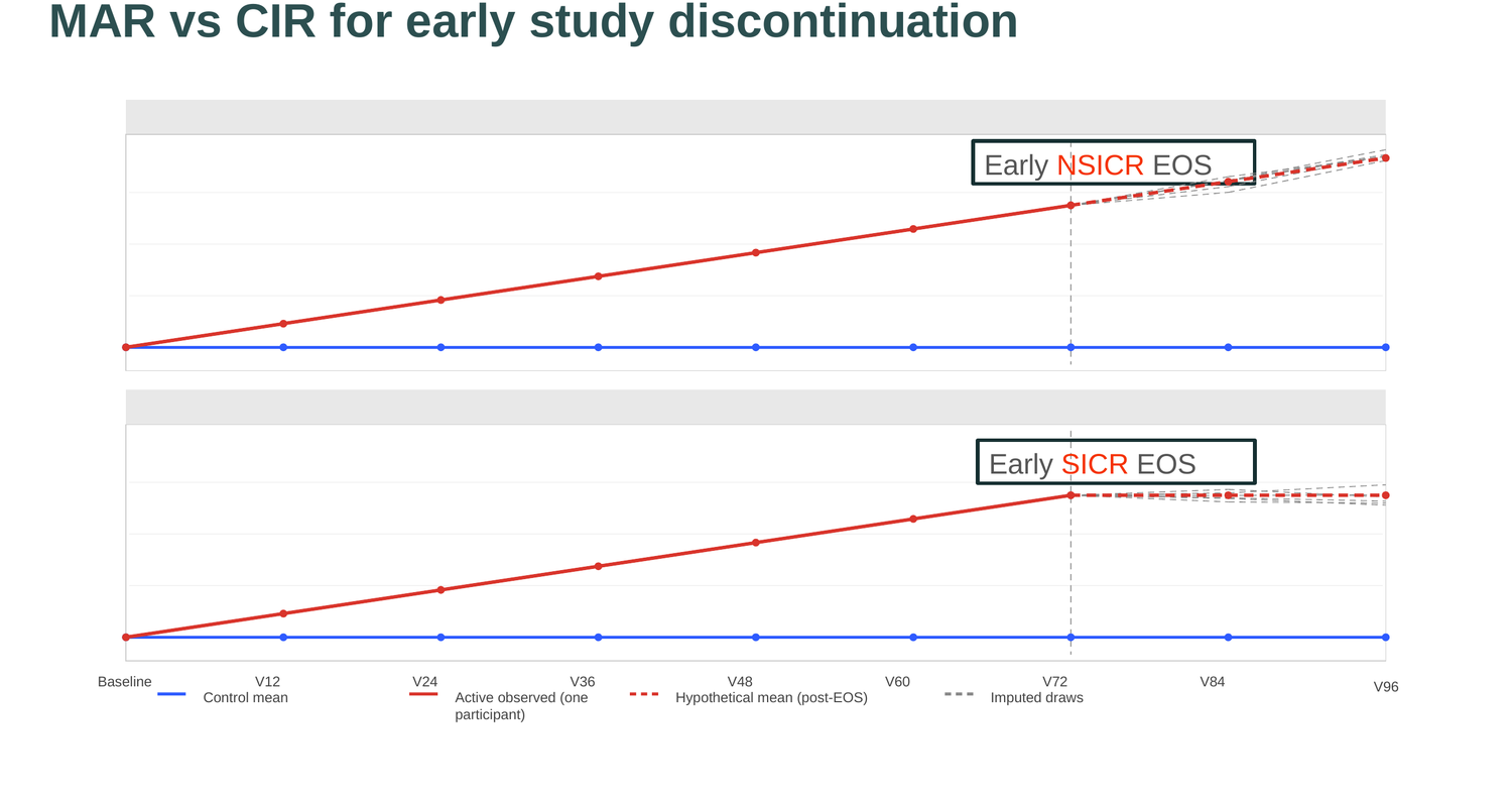
Under MAR the imputed trajectories keep climbing. Under CIR they flatten out, because the reference arm is not improving. CIR is more conservative than MAR.
Other reference-based assumptions exist, such as jump to reference (J2R) and copy reference (CR). Wolbers et al. evaluate those as well. We focus on CIR here.
Approach 1: Bayesian multiple imputation
This is the conventional route, and the one the five SAS macros of Carpenter and Roger made standard.
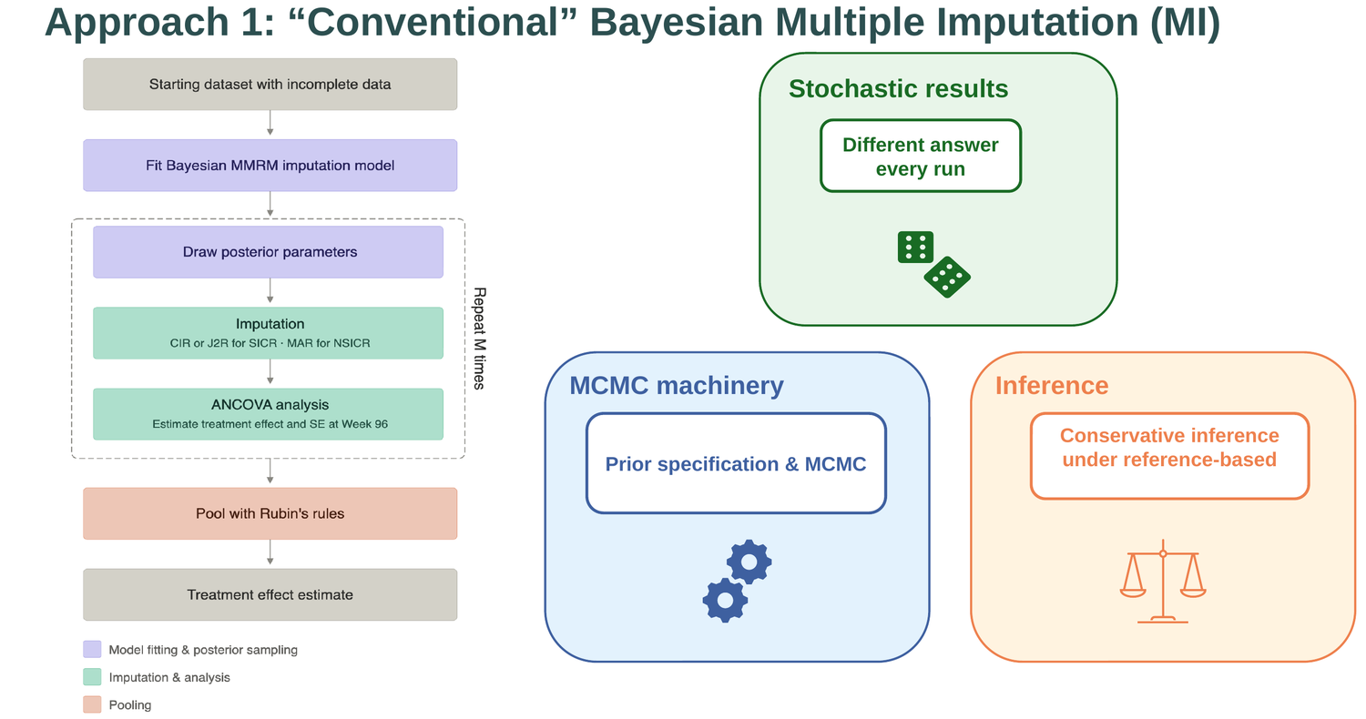
A Bayesian MMRM is fitted to the incomplete data. Parameters are drawn from the posterior, the missing values are imputed under the chosen assumption, an ANCOVA is run on each completed dataset, and the results are pooled with Rubin’s rules.
Two properties matter here. The procedure is stochastic, so the answer changes between runs unless the seed is fixed. And under reference-based imputation, Rubin’s rules do not estimate the frequentist repeated-sampling variance of the estimator. They estimate something larger. This is the issue we care about here: the inference becomes conservative, the type I error falls well below the nominal 5%, and we do not want to be too conservative because it has a cost in power! 🤯
Approach 2: conditional mean imputation with resampling
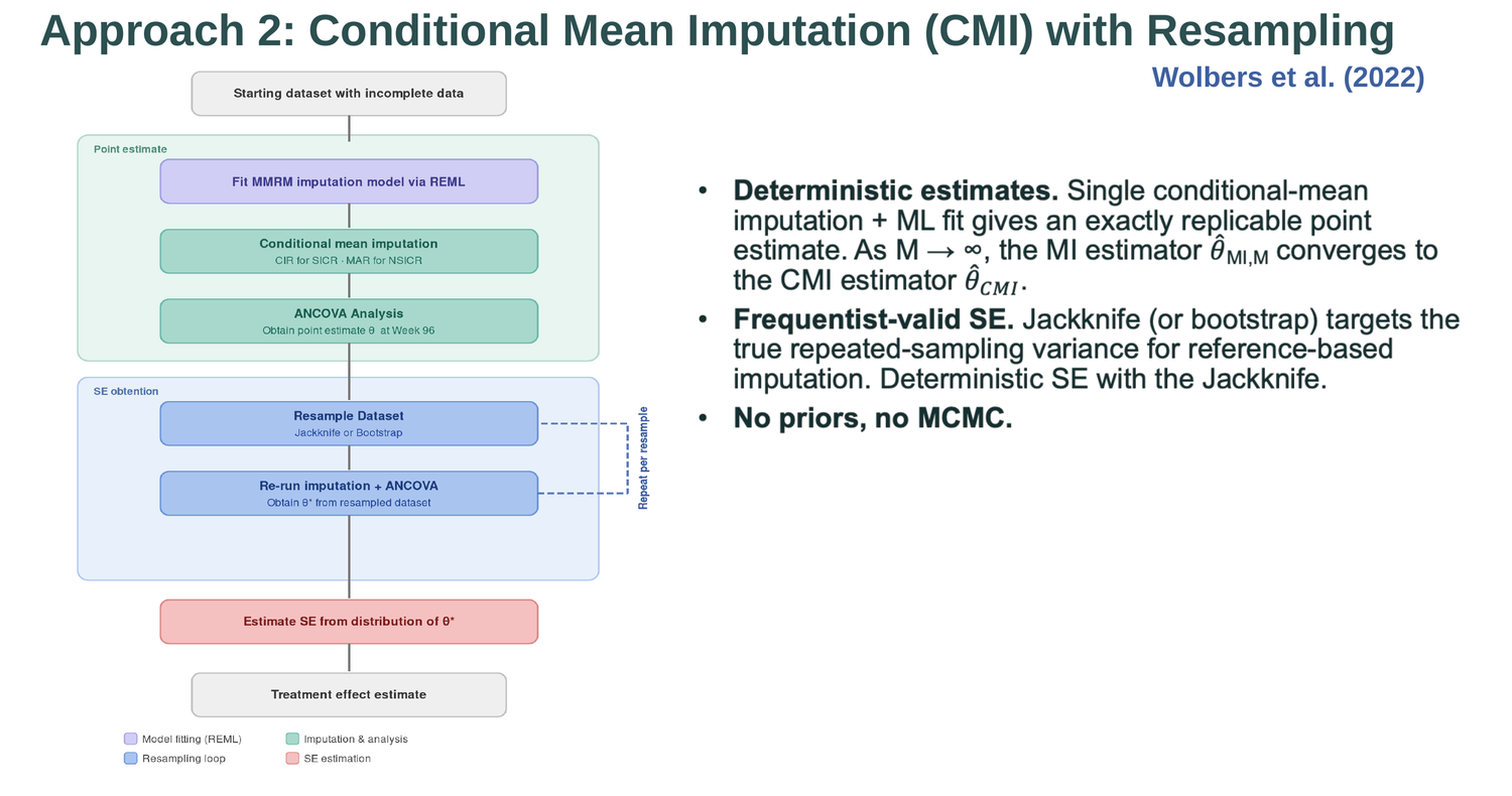
The point estimate is obtained differently. The MMRM is fitted by REML, each missing value is replaced by its conditional mean rather than a draw, and the ANCOVA is run once. There is no Monte Carlo noise, so the point estimate is exactly reproducible. As the number of imputations grows, the Bayesian MI estimator converges to this one.
The standard error then comes from resampling the whole procedure, by jackknife or by bootstrap, which asymptotically targets the repeated-sampling variance directly even in the reference-based imputation. No priors and no MCMC. With the jackknife even the standard error is reproducible, because the jackknife is deterministic. This is the approach of Wolbers et al. (Pharmaceutical Statistics 2022), implemented in the rbmi package on CRAN.
Why we considered it
In the simulations reported by Wolbers et al., with 100 participants per arm, the two approaches agree under MAR and separate under CIR.
| Setting | Bayesian MI | CMI + jackknife | CMI + bootstrap |
|---|---|---|---|
| Type I error under MAR | 5.0% | 5.0% | 5.0% |
| Type I error under CIR | 2.5% | 4.9% | 5.2% |
| Power under MAR | 92% | 92% | 92% |
| Power under CIR | 82.0% | 88.3% | 88.7% |
Under CIR the Bayesian type I error is 2.5% against a nominal 5%, and the cost is about six percentage points of power. The resampling methods recover it. This is an important gain in power! 🎉
One caution is already visible in the table. The bootstrap does not keep the type I error at 5%. The authors report exact type I error protection for the jackknife and slight inflation for the bootstrap.
Two things in that paper pointed straight at our setting:
- the simulations used 100 participants per arm, so behavior at a much smaller sample size was not evaluated;
- the authors note that the jackknife variance tends to be biased upwards in finite samples, whereas bootstrap variances are more susceptible to downwards bias.
The question we had was whether it still holds at the sample size of a rare disease trial. So I went over it 🚀
There is an interesting debate on which variance is the right target here, the information-anchored variance or the frequentist repeated-sampling variance. See the letter by Cro et al. (Pharmaceutical Statistics 2024) and the rejoinder by Wolbers et al. (Pharmaceutical Statistics 2024). We do not take a position on that discussion and we only look at how the methods behave at a small sample size 🙂.
Our simulation
10,000 longitudinal multivariate normal datasets under the null and under the alternative, at a total sample size of 42 with 2:1 allocation, so 28 against 14. Monte Carlo standard error at the 5% level is about 0.2% under the null and about 0.4% under the alternative.
Dropout is MAR with 15% probability and monotone. Missing values are imputed under both MAR and CIR, followed by an ANCOVA. Four methods are compared: Bayesian MI with 100 imputations, CMI with the jackknife, and CMI with the bootstrap at 1000 replicates using both the normal approximation and the percentile interval.
Type I error under the null
All four methods give unbiased point estimates. The differences are entirely in the standard error.
| Strategy | Method | Type I error (%) | SD of \(\hat\theta\) | Mean \(\widehat{SE}\) |
|---|---|---|---|---|
| MAR | Bayesian MI | 5.1 | 16.9 | 16.7 |
| CMI + jackknife | 4.6 | 16.9 | 17.6 | |
| CMI + bootstrap (normal) | 6.2 | 16.9 | 16.4 | |
| CMI + bootstrap (percentile) | 6.3 | 16.9 | — | |
| CIR | Bayesian MI | 3.8 | 16.0 | 16.8 |
| CMI + jackknife | 4.4 | 16.0 | 16.8 | |
| CMI + bootstrap (normal) | 6.1 | 16.0 | 15.7 | |
| CMI + bootstrap (percentile) | 6.2 | 16.0 | — |
Under CIR, Bayesian MI is conservative at 3.8%, exactly as expected. That part reproduces.
The resampling methods are a different story. Under MAR all three should agree, and they do not. The jackknife over-estimates the standard error (17.6 against an empirical 16.9) and is conservative at 4.6%. The bootstrap under-estimates it (16.4) and the type I error is inflated at 6.2%, so at this sample size it is not an option. The same pattern appears under CIR.
This is finite-sample bias in the resampling variance estimators, and at 42 participants it is large enough to matter.
Power under the alternative
| Strategy | Method | Power (%) | Δ vs Bayesian (pp) | Relative gain (%) |
|---|---|---|---|---|
| MAR | Bayesian MI | 82.8 | — | — |
| CMI + jackknife | 81.3 | −1.5 | −1.8 | |
| CMI + bootstrap (normal) | 85.0 | +2.2 | +2.7 | |
| CMI + bootstrap (percentile) | 84.5 | +1.7 | +2.1 | |
| CIR | Bayesian MI | 75.3 | — | — |
| CMI + jackknife | 77.8 | +2.5 | +3.3 | |
| CMI + bootstrap (normal) | 81.7 | +6.4 | +8.5 | |
| CMI + bootstrap (percentile) | 81.3 | +6.0 | +8.0 |
Under CIR the bootstrap does show the large power gain reported at bigger sample sizes, but at the cost of the inflated type I error shown in the previous section.
The jackknife gains 2.5 percentage points under CIR and loses 1.5 under MAR. That is a much smaller effect than the published results suggest, and it comes from the upward small-sample bias in its standard error.
How large does the trial have to be
I do still believe in the resampling methods, so the next question was when I would be able to use them. To be honest, this one came up only a few weeks before the presentation 🙂.
The finite-sample behavior is not caused by the imputation. To show that, we repeated the exercise on complete data, with nothing missing at all, across a range of sample sizes. 10,000 datasets per sample size, 2:1 allocation, ANCOVA.
The figure plots the type I error against the total sample size. The point estimate is the same ANCOVA fit throughout, so the three lines differ only in how the standard error is obtained: the ANCOVA model-based SE, and the SEs from jackknife and bootstrap resampling. The dashed line is the nominal 5%, the dotted lines are the Monte Carlo error band, and the vertical line marks the 42 participants used above. What to look for is where each line enters the band and stays there.
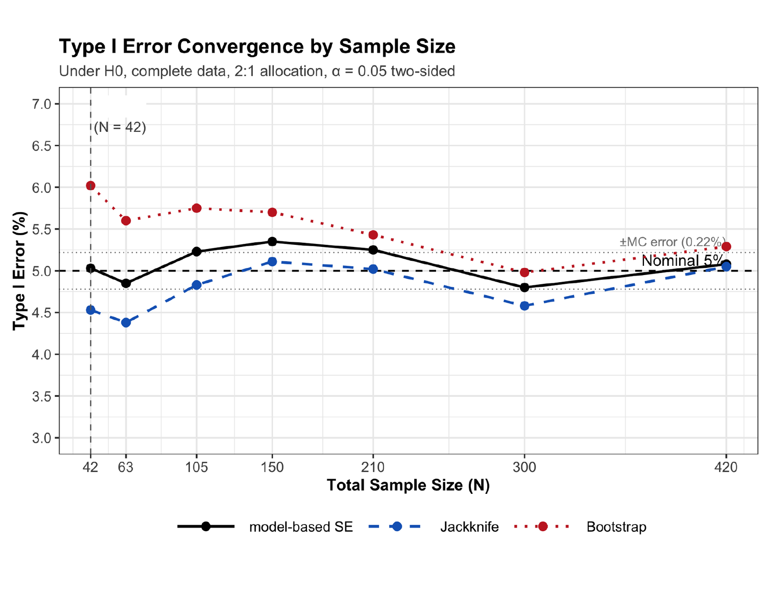
The bootstrap stays liberal until the total sample size reaches about 300. The jackknife settles down from about 150.
Wolbers et al. simulated 100 participants per arm, 200 in total, which is above that threshold, and they saw no small-sample bias. The two results line up 🙌
Since there is no missing data here, the imputation model plays no part. What the figure shows is the small-sample behavior of the resampling variance estimators themselves.
Conclusions
- In a rare disease trial, Bayesian MI still looks like the right default. The resampling alternatives show finite-sample bias in the standard error at small sample sizes.
- Bayesian MI is conservative under reference-based imputation. That is a real cost in power, but conservatism is the least concerning way for a method to fail. What should I say 🤷
- CMI with the jackknife is a promising deterministic alternative once the sample size is large enough. It controls the type I error correctly even under reference-based assumptions without being too conservative.
- Once I step out of rare disease, I will certainly give conditional mean imputation with the jackknife a try again 🙂