Simulating missing data

Biostats

Author

Imanol Zubizarreta

Published

February 25, 2024

Code

library(dplyr)
library(tidyr)
library(ggplot2)
library(mice)
library(forcats)
library(ggExtra)

Introduction

Missing data is one of the most important issues to consider when it comes to data/statistical analysis. Different methodologies have been proposed to deal with it and significant efforts on validating/evaluating them have been made. The starting step of these evaluations is usually simulating data accompanied by the missingness addition/simulation under different scenarios and different missing proportions. The action of adding missingness in your data set is called amputation and this very first step will be the main topic in this post. The scenario under which you will be generating missing data will be certainly the most important step in your simulations, thereby worth creating an amputation specific post. You will see, I am avoiding any clinical trial specific verbatim 🙂, as I want these starting posts to be domain agnostic.

Objectives

The primary objectives in this post are:

To go over the amputation process by the use of the great mice package. Let’s ignore the multivariate normal nature of many data sets that we use in clinical trials. Basic things can perfectly be explained by simulating very simple data sets.
To present the scenarios under which you will be simulating your missing data: Missing Completely at Random (MCAR), Missing at Random (MAR) and Missing not at Random (MNAR). Simple data sets also helpful to understand these concepts. You will certainly keep hearing about these three important concepts!

The secondary objectives are:

To share one of the findings I made when using the mice::ampute so that you can make sure you will not be doing this mistake when generating missingness.
Some deeper dive on what is going within mice::ampute and how this missing data is generated under the continuous probability distributions. mice::ampute enables you generating missing data under discrete probability distributions as well, by specifying the quantiles to be used for the “predictor” variables in the missing data generation process.

Generating the data sets

In the clinical trial setting, which is the main topic on my daily work, you may have longitudinal data, and you may certainly be willing to estimate the difference in the outcome between different treatment groups in an specific time point. However, for the seek of focusing on what we want to emphasize in this post, we will simulate very simple analysis data sets, as all the terms we will be talking about in this post are not clinical trial domain specific. These are the three variables we will be simulating for this post.

Subject variable.
Normally distributed age variable.
Outcome variable that is positively correlated with the age.

Code

subject <- paste(rep("SUBJ", 50), seq(1, 50), sep = "-")
set.seed(123)
age <- rnorm(50, 40, 10)
out <- 20 + 2 * age + rnorm(50, 0, 20)
anl <- data.frame(SUBJID = subject, AGE = age, OUT = out)
head(anl)

  SUBJID      AGE       OUT
1 SUBJ-1 34.39524  93.85686
2 SUBJ-2 37.69823  94.82552
3 SUBJ-3 55.58708 130.31676
4 SUBJ-4 40.70508 128.78221
5 SUBJ-5 41.29288  98.07033
6 SUBJ-6 57.15065 164.63071

Code

ggplot(anl, aes(AGE, OUT)) + 
  geom_point() + 
  theme_bw() +
  ggtitle("Outcome positively correlated with age")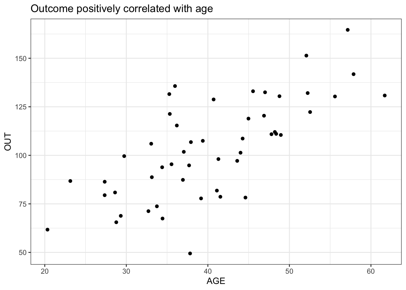

Simulating missing data in your data sets

Different missing proportions in the outcome variable will be simulated now based on the complete data set generated above, as these data sets will potentially be used in some later posts, where some evaluations will be made as a function of missing proportion.

In this post, and with the aim of keeping things simple, the outcome (OUT) variable will be the only variable at risk of facing missingness. The AGE variable will be always complete.

Types of missing data

Before we go into the amputation process, worth briefly presenting the three scenarios under which you can be generating missing data. We do not need complex/longitudinal data sets to understand these concepts:

Missing Completely At Random (MCAR): Probability of being missing does not depend in any other variable. In our specific case, imagine the missingness in the outcome OUT variable not depending in the age variable at all. All subjects would have the same probability of having the outcome variable missing. Working under MCAR makes life (amputation and imputation process) much easier, but not better, as unfortunately this assumption cannot be made in many cases 🤷.
Missing At Random (MAR): Probability of being missing in a certain variable is based on the values of another variable(s). In our case, imagine older subjects with a higher risk of having the outcome variable amputed. This is a quite typical assumption. Here keep in mind that the less correlated the age and the outcome are, MAR pattern will more reflect a MCAR missingness 🧐. Why? Because the less correlated they are, the more difficult will be for you to control and generate the conditional distributions of missingness on age. Once said this, you could even try different OUTCOME ~ AGE correlation levels and evaluate some of the analyses I will be doing in this and upcoming posts as a function of these correlation levels.
Missing Not At Random (MNAR): Probability of being missing in a certain variable is based on the variable itself. This scenario is the trickiest one when going over the imputation process. In clinical trials many times imputation is done under MAR (so that you can assume missing values depend on i.e some observed baseline characteristics) and then several sensitivity analyses are proposed address unverifiable missing data assumptions. Not a post to talk about this though 🙂.

Amputation by using mice::ampute

Let’s describe the main parameters of the mice::ampute function.

pattern: A matrix where you state all the different missing patterns in rows. The matrix should have as many columns as number of variables you have in the data set. In the following chunk of code, I am defining a one dimensional matrix which states the outcome as the only variable of being missing. In the real life scenarios you will be potentially foreseeing different missing patterns. Just keep adding as many rows with 1/0 as patterns you are planning for.

Code

pattern_missing <- matrix(c(1, 1, 0), nrow = 1)
colnames(pattern_missing) <- names(anl)
pattern_missing

     SUBJID AGE OUT
[1,]      1   1   0

mech: A string specifying the missingness mechanism, the previously defined MAR (by default), MCAR and MNAR. Let’s work under MAR.
weight: Under MAR (default option), the matrix that assigns values of 1 to the variables that remain complete in a certain pattern, and 0 to variables that will become incomplete, so that missingness is based on the observed variables. You can either add values between 0 and 1 into different variables in case you want the “predictor” variables of missingness to have different relative influence when determining the missingness. This will then be reflected in the weighted sum scores that we will briefly mention in the “deeper dive” section. In our simple example this is not a problem as missingness will depend merely on age. If you want to generate missingness under MNAR, the non-null value should be assigned to the variable itself and 0 to the remaining variables.

Code

#age being the only "predictor" of missingness
weights <- matrix(c(0, 1, 0), nrow = 1)
colnames(weights) <- names(anl)
weights

     SUBJID AGE OUT
[1,]      0   1   0

prop: Proportion of missingness you want to add in your starting complere data. In this post we will be creating different amputed data sets with different missing proportions.

Code

#20, 40, 60 and 80% of missing
missing_rates <- c(0.2, 0.4, 0.6, 0.8)

freq: A vector of length of number of patterns containing the relative frequency with which the patterns should occur. In our case we have a single pattern (outcome OUT missing while AGE remains complete), so not critical for us.

As commented before, we will be generating missingness under MAR, where, long story short, the older subjects will have a higher hazard of being missing as we are stating the parameter type = RIGHT, under a continuous probability distribution (we will later talk a bit more about it). You can either use the odds parameter if you want to use a quantile based likelihood of being missed by assigning different relative probabilities to each age quantile (do not forget to set the cont parameter to FALSE).

Let’s make use of the function now! Please make use of Rianne Margaretha Schouten et al for more details on the arguments of mice::ampute.

Code

#calling mice::ampute under different target missing proportions 
amputed_list <- lapply(missing_rates, FUN = function(missing_tmp) {
  set.seed(123)
  result <- mice::ampute(
    anl, prop = missing_tmp, 
    patterns = pattern_missing, 
    mech = "MAR", 
    weights = weights,
    type = "RIGHT")
})

#showing the first records of the amputed data set with 60% of missingness
amputed_list[[3]]$amp[1:10, ]

   SUBJID      AGE      OUT
1      NA 34.39524       NA
2      NA 37.69823       NA
3      NA 55.58708       NA
4      NA 40.70508       NA
5      NA 41.29288       NA
6      NA 57.15065       NA
7      NA 44.60916       NA
8      NA 27.34939       NA
9      NA 33.13147       NA
10     NA 35.54338 95.40559

Ups! mice::ampute() is converting the character variable SUBJID to NA. Let’s add the subject variable information again in the four amputed data sets (under the four different missing proportions).

Code

amp_df_list <- lapply(amputed_list, FUN = function(amp_tmp) {
  amp_tmp$amp %>%
    mutate(SUBJID = anl$SUBJID)
})

names(amp_df_list) <- c("prop20", "prop40", "prop60", "prop80")

amp_df_list[[3]][1:10, ]

    SUBJID      AGE      OUT
1   SUBJ-1 34.39524       NA
2   SUBJ-2 37.69823       NA
3   SUBJ-3 55.58708       NA
4   SUBJ-4 40.70508       NA
5   SUBJ-5 41.29288       NA
6   SUBJ-6 57.15065       NA
7   SUBJ-7 44.60916       NA
8   SUBJ-8 27.34939       NA
9   SUBJ-9 33.13147       NA
10 SUBJ-10 35.54338 95.40559

Let me check whether the amputation has been done under MAR assumption. Always good to check it out!

Code

breaks <- quantile(amp_df_list[[1]]$AGE, c(.33, .67, 1))
breaks <- c(0, breaks)
labels <- c('young', 'medium', 'old')

amp_df_bind <- do.call(rbind, amp_df_list) %>%
  bind_cols(
    miss_prop = rep(names(amp_df_list), each = nrow(amp_df_list[[1]]))
    ) %>%
  mutate(is_missing = ifelse(is.na(OUT), "Missing", "Not Missing"), 
         AGE_CAT = cut(AGE, breaks = breaks, labels = labels)) 

ggplot2::ggplot(amp_df_bind  , aes(x = AGE_CAT, fill = is_missing)) + 
  geom_bar() +
  facet_wrap(~ miss_prop) +     
  theme_bw()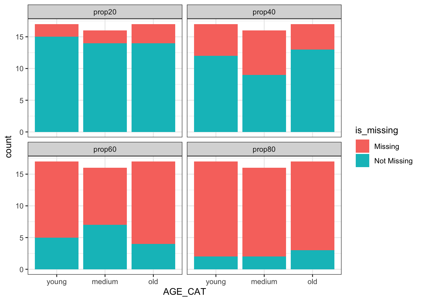

Not what we were expecting, right? Missingness in OUT variable is by no means dependant on the age variable 🤔, which was our original intent!

After digging into the inner functions from mice::ampute, I realized the user must remove the character variables such as SUBJID before going over the amputation process. Please see the issue I created in case you are interested in the details. Once said this, keep this in mind when you will be simulating missingness in your analysis data sets, as you may not be getting the intended missing distributions.

After going over the same process but removing the SUBJID variable, you can see the distributions make much more sense. Missingness does depend on age now. 🥇

       AGE      OUT SUBJID
1 34.39524 93.85686 SUBJ-1
2 37.69823       NA SUBJ-2
3 55.58708       NA SUBJ-3
4 40.70508       NA SUBJ-4
5 41.29288       NA SUBJ-5
6 57.15065       NA SUBJ-6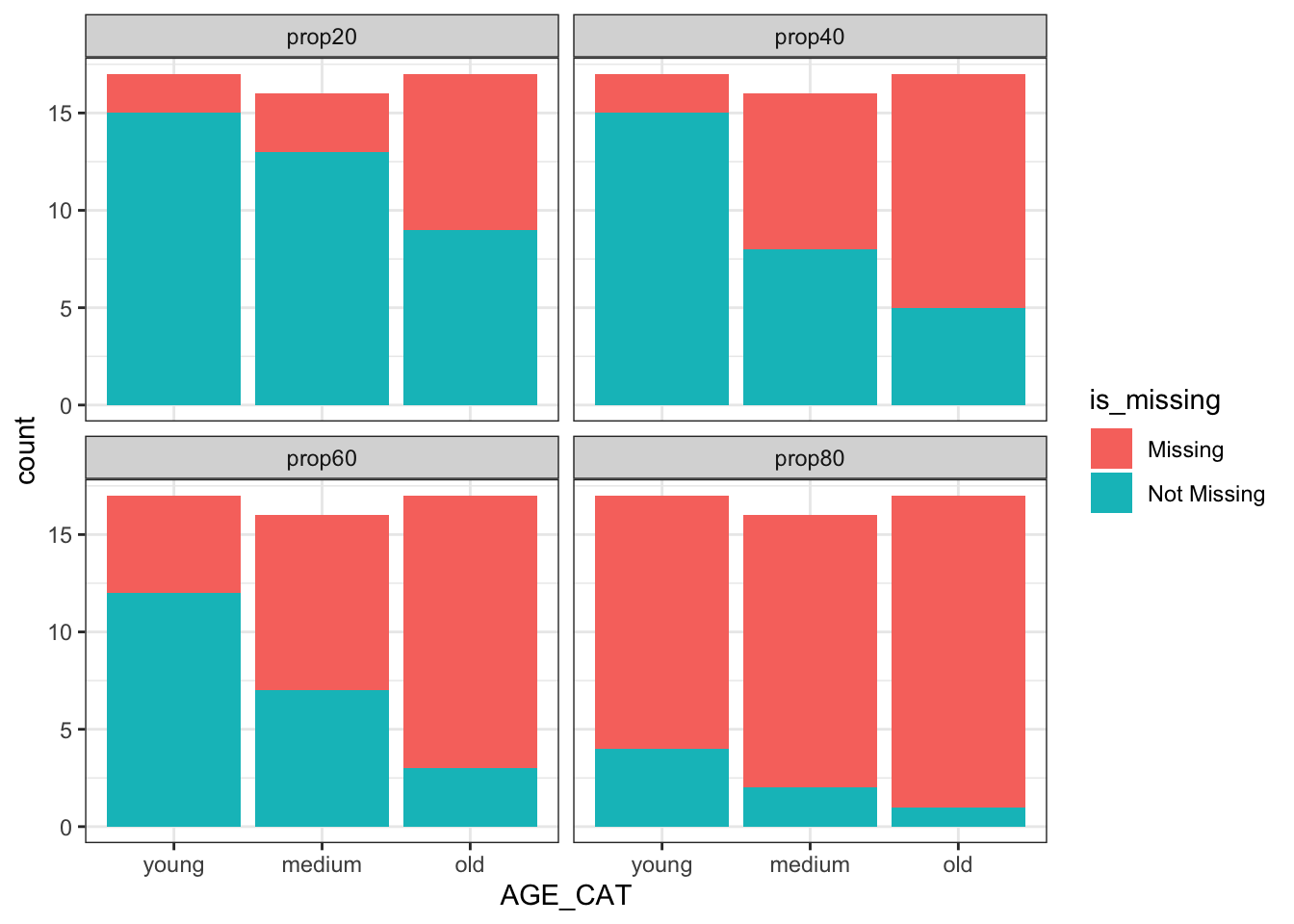

Some deeper details on the amputation

I would strongly recommend you going over Schouten et al. (1) (take your time on Figure 2) to understand how mice::ampute() works when there are more than one missing patterns (multivariate amputations). You will need to pay attention to freq parameter of the function.

Let’s mimic some of the steps mice::ampute is carrying forward.

Calculating weight sum scores

Worth mentioning the weighted sum scores which is defined by the following equation.

\[ wss_i = w_1*y_{1i} + w_2*y_{2i} + .... w_m*y_{mi} \]

Where:

i is an specific record in the data set.
\(w_1 ... w_m\) are the pre-specified weights for each predictor variable.
\(y_1 ... y_m\) is the set of variables in the data set.

As we have seen when defining the weight parameter under mice::ampute, we have only assigned a non-null weight (of value 1) to the variable AGE, as we were aiming to ampute the OUT variable under MAR assumption based on how old the subject is. The above equation would be very simple in this example (\(wss_i = w * AGE\)), where w = 1.

Continuous probability distributions for deciding on missingness

Last but not least, I would like to briefly talk and visualize the continuous probability distribution (logistic distribution) mice::ampute is generating to decide on the missingness. First we get the scaled weighted sum of scores.

Code

weights <- as.matrix(weights)
scaled_data <- scale(anl1)
scores <- c(scaled_data[, 1])

head(scores)

[1] -0.64250835 -0.28576479  1.64634862  0.03899559  0.10248111  1.81522403

By using the above scaled scores, we will be describing the probability of being missing by a logistic distribution function.

See in the following plot the pattern among the values of the weighted sum scores and associated probabilities of being missing. I color-coded by their original categorical AGE variable so that you can see the older subjects will be at higher risk of being amputed by the use of logistic distribution function. Empty points are the ones that mice::ampute converted them to missing in the above missing generation steps (under missing proportion rate of 40%).

We first generate the probabilities of being missing from our log-odds (weighted sum scores) values:

\[P(missing) = \frac{e^{x}}{1 + e^{x}}\]

Code

#using plogis to get the missing probabilities from exp(x)/(1 + exp(x))
p_missing <- plogis(scores)

p_missing_scores <- data.frame("p_missing" = p_missing, "scaled_wss" = scores) %>%
  bind_cols(AGE_CAT = amp_df_bind[51:100, c("AGE_CAT", "is_missing")])

ggplot(
  p_missing_scores, 
  aes(x = scores, y = p_missing, fill = AGE_CAT, color = AGE_CAT, shape = is_missing)
  ) + 
  geom_point(size = 3) + 
  scale_shape_manual(values = c(1, 19)) + 
  scale_size_manual(values = c(2)) + 
  theme_bw()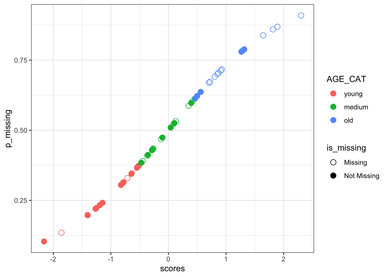

Then we go over the Binomial random variate generation by the use of the probabilities obtained above, where we will be obtaining the target missing cases.

Code

set.seed(123)
is_missing <- rbinom(n = length(scores), size = 1, prob = p_missing)
head(data.frame(p_missing, is_missing))

  p_missing is_missing
1 0.3446797          0
2 0.4290410          1
3 0.8383969          1
4 0.5097477          0
5 0.5255979          0
6 0.8599921          1

mice::ampute and specifically the inner mice::ampute.continuous function goes over a very similar approach but it deals with the so called shifted probability distributions to try to solve the following two issues:

To keep the joint missingess percentages similar to the target missing proportion when dealing with multivariate missingness (See Appendix 2 from Schouten et al. (1)).
To better distribute the missingness, as cases with extreme missing predictor values (AGE in our case) will have P(missing) = 0.99 (asymptotic function. Shifting the probability curve, you can somehow prevent for this.

Binary search algorithm to find the shift parameter

Code

missing_cases_no_shift <- c()
for (i in 1:100) {
  missing_cases_no_shift[i] <- sum(rbinom(n = length(scores), size = 1, prob = p_missing))
}

missing_cases_no_shift <- mean(missing_cases_no_shift) / 50 * 100

Running the above random generation for the binomial distribution 100 times, we are obtaining a mean proportion of missingness of 51 % (centered at P = 0.5). Then, how does mice::ampute achieve the proportion of missingness assigned by the user? For instance, our target proportion of missingness were 20, 40, 60 and 80%. We need to get the correct shift \(\delta\) parameter so that we can move the probability curves in the y axis.

\[P(missing) = \frac{e^{x + \delta}}{1 + e^{x + \delta}}\]

This can be achieved by the binary search algorithm, and this is how mice::ampute behaves. For the target missing proportion of 60%, the \(\delta\) obtained with the binary search algorithm is of 0.492. Let’s now plot the non-shifted and the shifted probability distributions in the same figure.

Code

shift <- 0.492

p_missing_shift <- plogis(scores + shift)

p_missing_scores_shift <- data.frame("p_missing" = p_missing_shift, "scaled_wss" = scores) %>%
  bind_cols(AGE_CAT = amp_df_bind[51:100, c("AGE_CAT", "is_missing")]) %>%
  mutate(type = "shifted curve")

p_missing_all <- p_missing_scores_shift %>%
  bind_rows(p_missing_scores %>%
              mutate(type = "non-shifted curve"))

ggplot(
  p_missing_all, 
  aes(x = scaled_wss, y = p_missing, color = type, group = type)
  ) + 
  geom_line() + 
  theme_bw() +
  xlab("Scaled Weighted Sum Scores") +  # for the x axis label
  ylab("Probability of converting to Missing")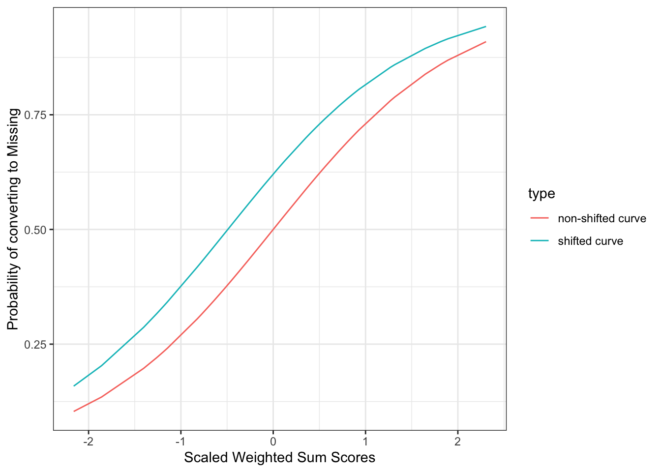

Code

missing_cases_shift <- c()

for (i in 1:100) {
  missing_cases_shift[i] <- sum(rbinom(n = length(scores), size = 1, prob = p_missing_shift))
}

missing_cases_shift <- mean(missing_cases_shift) / 50 * 100

Finally, going now over the random generation process from binomial distribution 100 times, we now successfully achieve a mean value of 60% of missingness! 😎

Summary

See the main points we have worked on during this post:

Presented the 3 scenarios (MCAR, MAR, MNAR) under which you can simulate missingness.
Showcased the mice::ampute function for simulating missingness, by mainly focusing on the missingness under MAR. We simulated the complete data and generated 4 data sets with 4 different missing proportions (20, 40, 60, 80%). The data sets will be used in the next post, so stay tuned!
Highlighted the need of excluding the character variables (i.e the subject id) before going over the amputation process. Otherwise, your target missing distributions will not be achieved!
Made a deeper dive over the mice::ampute functionality with the use of continuous probability distributions, by demistifying and visualizing some of the internal steps and results that the function generates to get the final distribution of missingness with the target proportion and mechanism (we worked under MAR).

Sharing a picture that I took this weekend at Uetliberg (Zurich, Switzerland). Nice walk and views of the Swiss Alps that helped me putting some of my ideas in order to properly finalize this writing. 😃

See you in the next post!

References

R. M. Schouten, P. Lugtig, G. Vink, Generating missing values for simulation purposes: A multivariate amputation procedure. Journal of Statistical Computation and Simulation 88, 2909–2930 (2018).