Equal vs. Proportional Weighting in Least-Squares Means
Introduction
In clinical trials, least-square means (LSMs) or marginalized means are often used to summarize adjusted treatment effects after fitting a model that includes prognostic covariates.
These model-based means average predicted outcomes across subgroups defined by covariates (e.g. disease severity), but, How should these marginal means be averaged across covariate levels?
In R, the emmeans() function is a widely used tool for computing LSMs. It offers two common weighting options for averaging over covariates:
"equal"weighting: averages subgroup means equally (e.g., assumes 50% Severe, 50% Non-Severe),"proportional"weighting: uses the observed distribution of the covariates/baseline characteristics in the sample (e.g., Disease severity: 20% Severe, 80% Non-Severe).
By default, emmeans() uses equal weighting and SAS LSMeans has the same default weights setting . Since this choice can affect the estimated marginal treatment effect, especially when covariates are prognostic or predictive, I decided to explore this topic in more detail in this post.🕵
Disclaimer
The purpose of this post is to characterize the relative performance of equal vs. proportional weighting in emmeans() when estimating marginal treatment effects, under varying levels of prognostic and predictive strength of a covariate. We are not attempting to characterize other sources of bias or imprecision that can arise in practice, such as unbalanced covariate distributions between treatment arms (which can inflate variance), inclusion of non-prognostic covariates that over-parameterize the model or bias due to model misspecification.
Prognostic vs. Predictive Covariates
Before diving into the examples, it is helpful to clarify what we mean by prognostic and predictive covariates in a clinical trial context:
A prognostic covariate is a patient characteristic that predicts the outcome of a disease regardless of the intervention, such as age or disease severity.
A predictive covariate modifies the treatment effect itself, meaning treatment effects differ across covariate levels.
Definition of bias in this post
Throughout this post, bias refers to deviation from the estimand of interest, that is in many cases, the treatment effect expected under the actual observed covariate distribution.
Scenario 1: Single-Arm Trial (No Control Group)
Imagine a single-arm trial where we wish to estimate the mean change from baseline in a continuous endpoint, adjusting for severity (Severe vs. Non-Severe), which is a baseline characteristic. In a real analysis, you would typically also adjust for baseline value and other prognostic variables, which can narrow confidence intervals by reducing residual variability. Here, for simplicity, we focus only on the severity covariate adjustment.
The estimand of interest is the mean change from baseline in the population actually enrolled in the study, that is, averaged over the observed distribution of severity levels.
Suppose:
- Severe cases are rare (e.g., 20% Severe)
- Severity is strongly prognostic
We fit a linear model adjusting for severity.
\[ \overline{\text{CHG}} = \beta_0 + \beta_2 \cdot \text{SEVERITY} + \epsilon \] Where \(\beta2\) represents the effect for the severe group relative to non-severe. We will reserve \(\beta1\) for the treatment effect term in the two-arm trial introduced later.
We compute the marginal mean across severity levels using both equal and proportional weighting.
Equal weighting (50% Severe, 50% Non-Severe):
\[ \text{Marginal Mean}_{\text{equal}} = \beta_0 + 0.5 \times \beta_2 \]
where 0.5 reflects the assumption of 50% Severe cases.
Proportional weighting (5/25 Severe):
Given that 5 out of 25 patients are Severe (20% Severe):
\[ \text{Marginal Mean}_{\text{proportional}} = \beta_0 + 0.2 \times \beta_2 \]
where 0.2 reflects the observed severity proportion in the study.
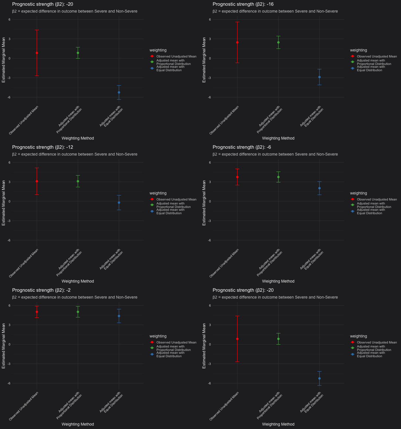
See below how the marginalized mean estimates evolve as the severity covariate becomes more or less prognostic. Each frame corresponds to a different prognostic strength, from non-prognostic (severity has no impact on outcome) to strongly prognostic (severity drives much worse outcomes).
These results are based on simulated data, where I varied the prognostic effect of the severity covariate (i.e., the magnitude of the coefficient β₂ in the model) to illustrate how the weighting choice affects the estimated marginal means and their uncertainty.

Unadjusted vs. proportional weighting (red vs green): The point estimate of the marginalized mean assuming the proportional distribution of the severity covariate should be very closely aligned with the unadjusted (observed) mean. The difference lies in the confidence interval. As severity becomes more prognostic, adjustment for it reduces residual variance, resulting in narrower confidence intervals. When severity is not prognostic, both the unadjusted and proportional means, including their confidence intervals, coincide.
Proportional vs. equal weighting (green vs blue): When severity is strongly prognostic, the equal-weighting LSMs (which assume a 50/50 Severe and Non-Severe distribution) become negatively biased, showing a worse mean outcome (where a lower value indicates worse performance) compared to the unadjusted and proportional means. This pattern appears under the assumption that only 20% of patients are Severe in the population. In addition, you may observe that the confidence intervals are broader when using equal weighting than when using proportional weighting. Without going into the math, this happens because the weighting applied to the variance of the coefficient estimates also changes. Equal weighting gives more influence to underrepresented subgroups, making the estimated marginal mean less efficient and leading to wider confidence intervals.
Scenario 2: Randomized-Controlled Trial with a Prognostic and Predictive Covariate
Now imagine a two-arm randomized controlled trial comparing Treatment vs Placebo, with a continuous endpoint defined as change from baseline.
In this setting, the estimand of interest is the difference in mean change from baseline between Treatment and Placebo, averaged over the population actually enrolled in the trial (i.e., under the observed covariate distribution).
In these simulations, we assume that 80% of patients are Severe and 20% are Non-Severe overall, across arms.
Severity is both prognostic (associated with outcome regardless of treatment) and predictive (the treatment effect differs between severity levels).
We will consider two cases:
Case 1: No Treatment by severity interaction
Model:
Without interaction, the model is:
\[ \overline{\text{CHG}} = \beta_0 + \beta_1 \cdot \text{TRT} + \beta_2 \cdot \text{SEVERITY} + \epsilon \]
In this setup, we can examine how the choice of weighting scheme (“equal” vs “proportional”) affects the least-squares means (LSMs) and the estimated treatment contrast.
Predicted least-squares means (LSMs):
- Treatment group:
\[ \text{LSM}_{\text{Treatment}} = \beta_0 + \beta_1 + w_{\text{S}} \cdot \beta_2 \]
- Placebo group:
\[ \text{LSM}_{\text{Placebo}} = \beta_0 + w_{\text{S}} \cdot \beta_2 \]
Thus, the treatment contrast is:
\[ \text{Treatment Difference} = (\beta_0 + \beta_1 + w_{\text{S}} \cdot \beta_2) - (\beta_0 + w_{\text{S}} \cdot \beta_2) = \beta_1 \]
And thereby, the treatment contrast is exactly \(\beta_1\), independent of \(w_{\text{s}}\). Weighting approach will not impact here.
Note: If the covariate is predictive, then the model without an interaction term is misspecified and will yield biased treatment estimates. Our focus here is only to compare the relative performance of the two weighting schemes, so model misspecification is not a topic for today 😬
Case 2: Treatment by severity interaction
Model:
\[ \overline{\text{CHG}} = \beta_0 + \beta_1 \cdot \text{TRT} + \beta_2 \cdot \text{SEVERITY} + \beta_3 \cdot (\text{TRT} \times \text{SEVERITY}) + \epsilon \]
The treatment contrast becomes:
\[ \text{Treatment Difference} = \beta_1 + w_{\text{S}} \times \beta_3 \]
where \(w_{\text{s}}\) is the weight assigned to Severe cases (depends on equal vs proportional weighting).
- Equal weighting uses \(w_{\text{s}}\) = 0.5 (by assumption),
- Proportional weighting uses \(w_{\text{s}}\) = observed Severe proportion in the trial.
Thus, the treatment contrast will differ based on the severity distribution and the weighting scheme used.
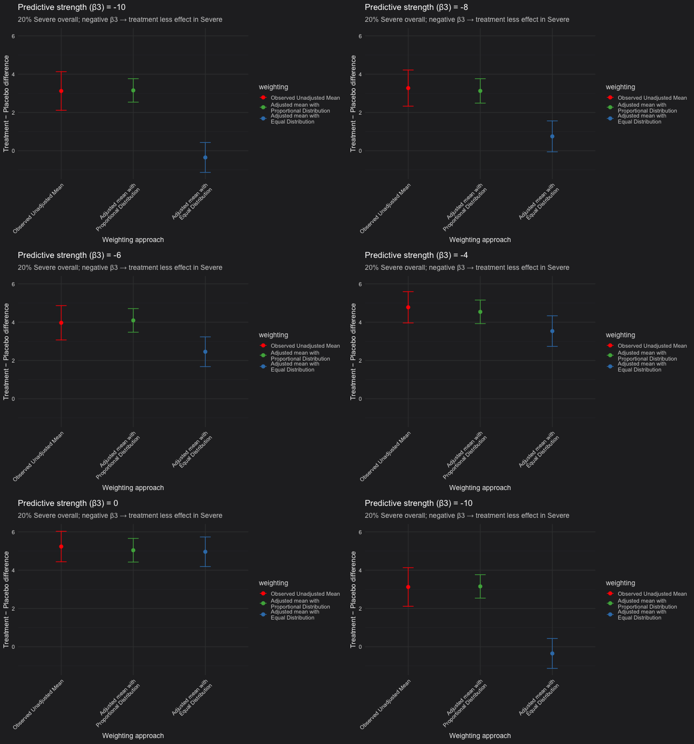
In this example, I simulated a randomized controlled trial with a predictive covariate (disease severity) and made Severe cases represent 20% of the population. The outcome model included a treatment × severity interaction (β₃), which controls the treatment effect heterogeneity between Severe and Non-Severe patients:
Simulation setup
- Non-severe patients have better outcomes overall (covariate is prognostic).
- Treatment performs better for non-severe patients (covariate is predictive).
- We fixed 20% of participants as Severe and varied \(\beta_3\) (treatment effect in the severe patients) from 0 (i.e not predictive) to −10 (strongly predictive).

- Unadjusted vs. proportional weighting (red vs green): When the covariate (severity) is prognostic but not predictive (β₃ = 0), the unadjusted and proportional LSM estimates are nearly identical. Confidence intervals from the proportional model are consistently narrower than those from the unadjusted analysis. This occurs because the model accounts for the prognostic covariate (β₂ ≠ 0), thereby reducing residual variance, even though β₃ = 0.
- Proportional vs. equal weighting (green vs blue): When the covariate is only prognostic, both weighting approaches yield the same expected treatment estimate. When the covariate is predictive, the equal-weighted LSM will deviate from the proportional one because it overrepresents the less common severe subgroup. In our simulation setting (20% of the patients are severe only), equal weighting can produce a downward-biased estimate
Conclusions
Under the assumption that the estimand of interest is the average treatment effect expected under the actual observed covariate distribution:
- In a single-arm setting, equal weighting can produce biased results whenever the covariate is prognostic, because the equal-weighted mean assumes an artificial 50/50 subgroup composition rather than the observed one.
- In a two-arm setting, equal weighting leads to bias when the covariate is predictive, that is, when the treatment effect differs across covariate levels.
- Equal weighting can also lead to wider standard errors and confidence intervals.
In practice, some studies intentionally apply enrollment caps to certain subgroups. In such cases, the resulting estimates reflect the realized composition of the randomized sample and would typically be described as trial-specific in the estimand definition. However, when a covariate distribution becomes unexpectedly unbalanced, neither by design nor representative of a target population, proportional weighting may not be totally justified.
All that said, when targeting proportional weights, remember to set the weights argument in emmeans() accordingly 😉.
Photo from a recent hike to Harder Kulm
