Understanding the use of the geometric mean in the context of clinical trials
Biostats
Author
Imanol Zubizarreta
Published
November 26, 2023
Introduction
Immunologic data, such as anti-drug antibodies (ADA) titers, IgE, or other dilution factor based assays tend to have positively skewed distributions with a long tail of larger values. When analyzing PK data, both drug concentration data and pharmacokinetic parameters usually follow a skewed distribution among patient population as well.
For instance, when analyzing the antibodies, a sample is taken from the patient blood and is then challenged with known antigens to detect the presence of antibodies to these antigens. A titer is a measure of how much a sample can be diluted before antibodies can no longer be detected. Titers are usually expressed as ratios, such as 1:256, meaning that one part serum to 256 parts saline solution (dilutant) results in no antibodies remaining detectable in the sample. A titer of 1:8 is, therefore, an indication of lower numbers of bacteria antibodies than a 1:256 titer. Once said this, how to analyze this data❓🤔
This can be a clear example of log-normally distributed data in the clinical trial setting!
Several laboratory biomarkers are many times visualized in a log scale, due to the log-normal nature of their conditional distributions as well, or because the percent or relative change is of more interest than the raw change. You will better understand this statement with some later examples.
The above renders analyses based on normal distribution theory questionable (i.e. t-tests and analysis of variance), as it distorts the sample mean as a measure of central tendency. These problems can be addressed through the analysis of log-transformed data. Data analyzed in this fashion are usually summarized with the geometric mean.
Generating lognormal longitudinal data
First of all, I am creating some subject level longitudinal data with the popular MASS::mvrnorm() function, widely used if you need to go over some simulations for your MMRM analysis. 🙂 Since MASS::mvrnorm() creates multivariate normal data, I am exponentiating the dummy data so that we can obtain our desired log-normal data conditional on different time points (baseline, Visit 1, Visit 2 and Visit 3). See some of the dummy data created. I tried visit 1 data to be very similar to the baseline with the aim of getting non-meaningful changes from baseline at this first visit.
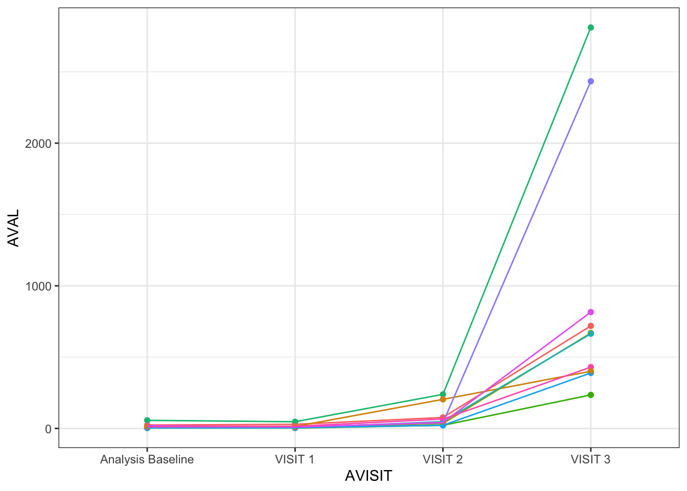
Due to its time/visit conditional log-normal nature of the dummy data generated, it is challenging to actually see the subject level trends over time. For the following visualizations, I will be creating a data set with extreme values, with pronounced shifts between visits.
Code
show_subjs <-unique(anl_long$SUBJID)[1:10]f_linear <-ggplot(data = anl_long2 %>%filter(SUBJID %in% show_subjs), aes(x = AVISIT, y = AVAL, color = SUBJID, group = SUBJID) ) +geom_point() +geom_line() +theme_bw() +theme(legend.position ="none")f_linear
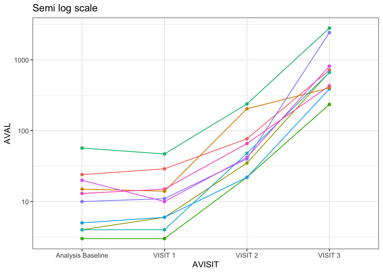
See now how well we can identify the trends when showing the same data in the log scale! 🕺
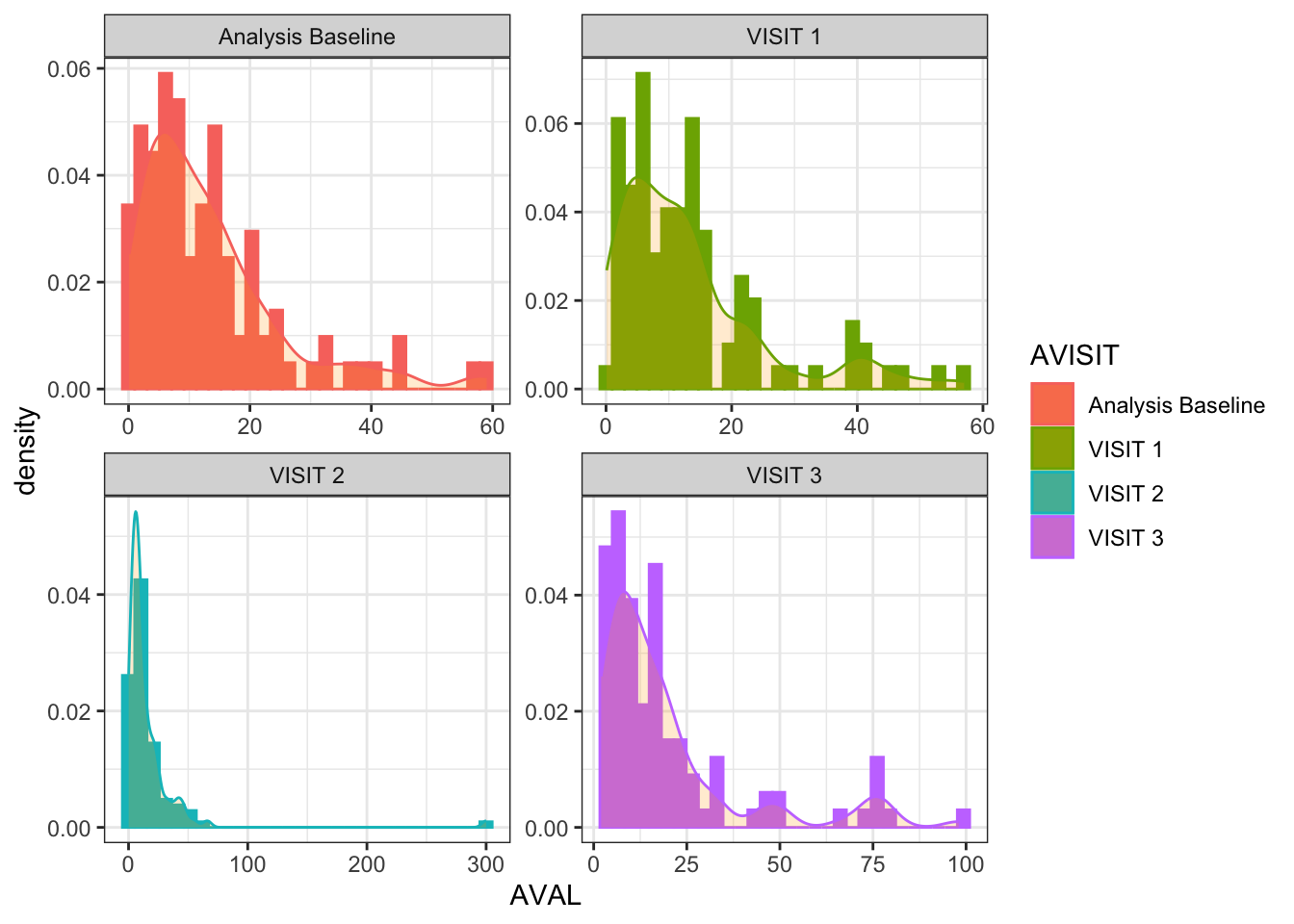
See the conditional log-normally distributed dummy data.
Code
ggplot(data = anl_long, aes(x = AVAL, color = AVISIT, fill = AVISIT)) +facet_wrap(~ AVISIT, scales ="free") +geom_histogram(aes(y = ..density..)) +geom_density(alpha =0.2, fill ="orange") +theme_bw()
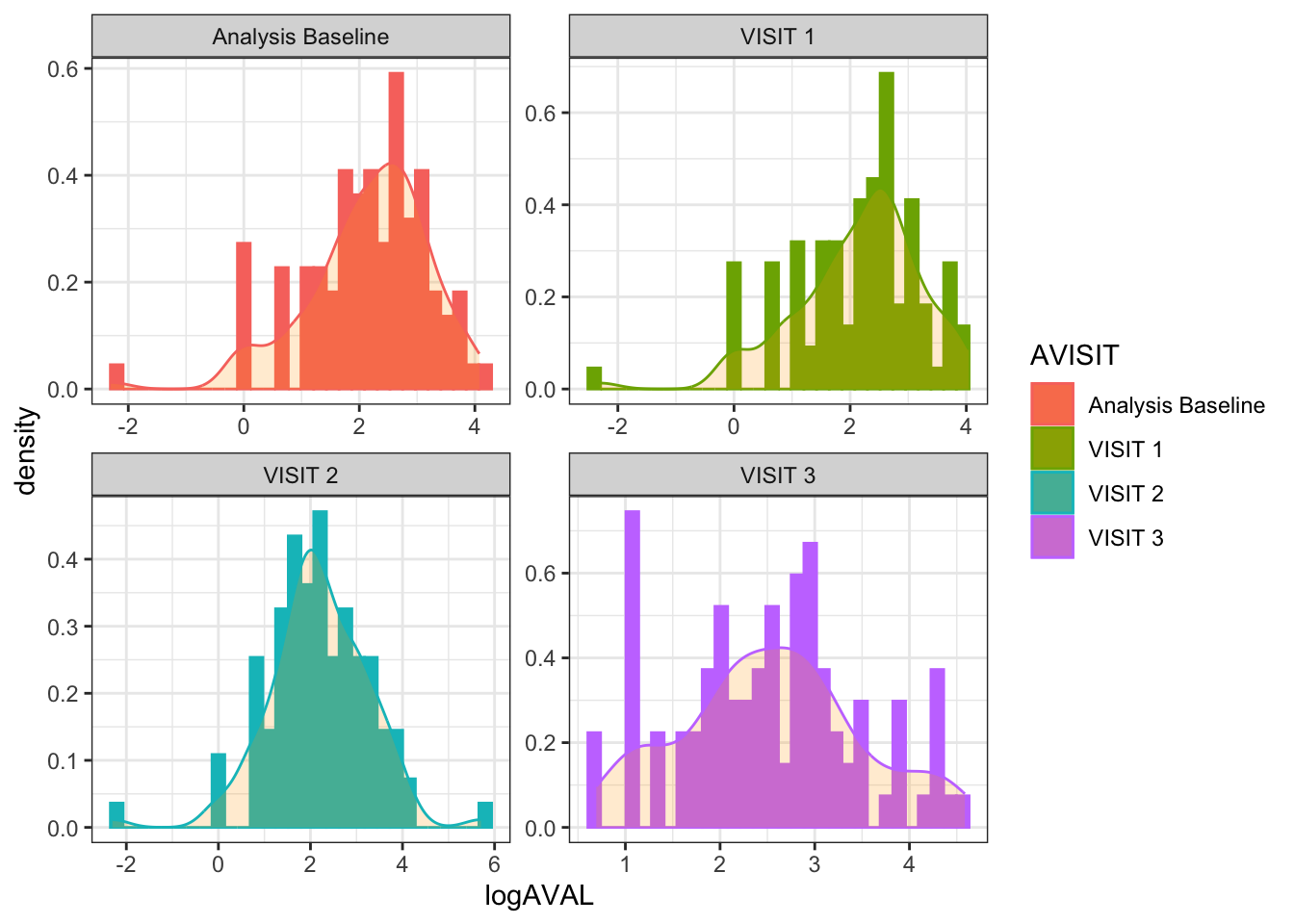
If we log-transform the AVAL values the distributions are much closer to the normal distribution:
Code
anl_long_log <- anl_long %>%mutate(logAVAL =log(AVAL))ggplot(data = anl_long_log, aes(x = logAVAL, color = AVISIT, fill = AVISIT)) +facet_wrap(~ AVISIT, scales ="free") +geom_histogram(aes(y = ..density..)) +geom_density(alpha =0.2, fill ="orange") +theme_bw()
Use of fold change or percent change
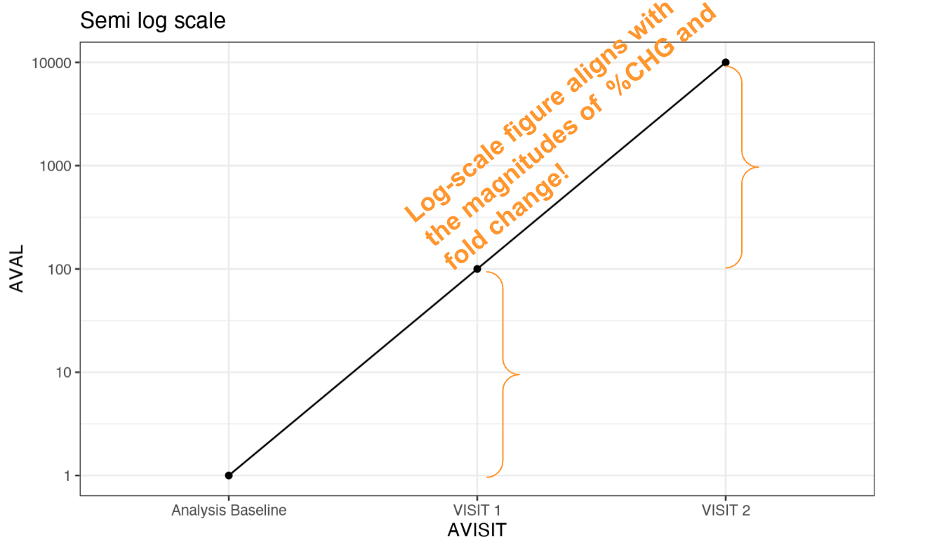
In the log-normally distributed data, the fold change or the percent change is of more interest than the raw change. See the following “edge” example I created with values of 1, 100 and 10000 at baseline, visit 1 and visit 2, respectively. These correspond to a fold changes of 100 and 10000 respectively, which yields to percent changes of 100% and ~10000% respectively. We have a fold change of 100 between visit 2 and visit 1.
When showing these values in a log10 scale, you will see the distances are exactly aligned with the magnitude of the fold changes! This does not happen when visualizing the data in the linear scale.
And we can link the above visual representation with the interpretation of the slope’s coefficients when going over a linear regression model where the dependant variable is log-transformed. In this case, the coefficient explains approximately a proportional or relative change for a given absolute change in the dependant variable.
Summarizing the values
When summarizing these log-normal values by analysis visit, the geometric mean should be used rather than the arithmetic mean. See the differences between the arithmetic mean and the geometric mean.
And what if we want to summarize the change from baseline? For the log-normally distributed data, it makes more sense summarizing the fold change or the percent change. See the next code chunk where change (CHG), percent change (PCHG) and fold change (FCHG) are calculated.
I used the Tern package for creating the below clinical trial reporting-ready table. Tern is an R package that contains analysis functions to create tables and graphs used for clinical trial reporting. Tern depends on rtables, which is the package that provides a framework for declaring complex multi-level tabulations and then applying them to data. These packages along with teal and teal.modules.clinical are a real game changer. You may think I am bit biased here, as I worked on the development of these packages for one year and a half (mind-blowing experience for my personal growth, have to say), but trust me, these packages are pure gold! 👑
Okay, coming back to the analysis, you can see the arithmetic and the geometric means are quite different. Arithmetic mean should not be used in the log-normal data as we are facing in this post. Then we should not either pay attention to the one sample t-test based p-values we are getting in the tables for the arithmetic means.
Code
t_summary_aval_chg <-basic_table(title ="Summary of the observed values") %>%split_cols_by("AVISIT") %>% tern::analyze_vars(vars =c("AVAL", "FCHG"), .stats =c("n", "mean", "mean_ci", "mean_pval", "range", "geom_mean", "geom_mean_ci"),.labels =c(n ="n", mean ="Arithmetic mean" , mean_ci ="Arith mean 95%CI", mean_pval ="Arith mean P-val", range ="Range", geom_mean ="Geometric mean",geom_mean_ci ="Geometric Mean 95%CI") ) %>%build_table(df = anl_chg) t_summary_aval_chg
Summary of the observed values

————————————————————————————————————————————————————————————————————————————————————————————
                         Analysis Baseline      VISIT 1          VISIT 2         VISIT 3
————————————————————————————————————————————————————————————————————————————————————————————
AVAL
  n                             100               100              100             100
  Arithmetic mean              13.3               13.4            16.2             19.5
  Arith mean 95%CI        (10.91, 15.63)     (10.96, 15.83)   (9.99, 22.47)   (15.47, 23.61)
  Arith mean P-val            <0.0001           <0.0001          <0.0001         <0.0001
  Range                     0.1 - 59.0         0.1 - 57.0      0.1 - 300.0      2.0 - 98.0
  Geometric mean                8.6               8.5              8.8             12.6
  Geometric Mean 95%CI     (7.00, 10.67)     (6.86, 10.56)    (7.12, 10.99)   (10.45, 15.20)
FCHG
  n                             100               100              100             100
  Arithmetic mean               1.0               1.2              2.8             5.3
  Arith mean 95%CI         (1.00, 1.00)       (0.99, 1.46)    (1.36, 4.16)     (1.38, 9.31)
  Arith mean P-val            <0.0001           <0.0001          0.0002           0.0087
  Range                      1.0 - 1.0         0.1 - 10.0      0.0 - 55.0      0.1 - 180.0
  Geometric mean                1.0               1.0              1.0             1.5
  Geometric Mean 95%CI     (1.00, 1.00)       (0.87, 1.11)    (0.79, 1.33)     (1.11, 1.91)
If we want to test i.e the mean change from baseline, doing this under the original non-transformed log-normal distribution would not be the correct approach. Let’s work under the log transformed values then! By using some of the log properties, we get the following:
i = 1….n; n being the number of subjects j = 1… 3; referring to the three post baseline visits where the change will be analyzed.By following the logarithmic properties, we can say that the change in log-transformed values is the same as the log of the fold change.
We already have the fold change values under the FCHG variable! Let’s log transform the fold changes then and save the values under the logFCHG variable.
How to test the change at each visit?
Now that we have the logFCHG values, we can summarize these logarithmic fold changes by also testing the mean against the null hypothesis that there is no change from baseline.
Code
t_summary_logfchg <-basic_table(title ="Summary of the log of the fold changes (logFCHG)") %>%split_cols_by("AVISIT") %>% tern::analyze_vars(vars =c("logFCHG"), .stats =c("n", "mean", "mean_ci", "mean_pval"),.formats =c(mean_pval ="x.xxxx | (<0.0001)")) %>%build_table(df = anl_chg2) t_summary_logfchg
Summary of the log of the fold changes (logFCHG)

——————————————————————————————————————————————————————————————————————————————————————————————
                              Analysis Baseline      VISIT 1         VISIT 2        VISIT 3
——————————————————————————————————————————————————————————————————————————————————————————————
n                                    100               100             100            100
Mean                                 0.0              -0.0             0.0            0.4
Mean 95% CI                     (0.00, 0.00)      (-0.14, 0.11)   (-0.24, 0.29)   (0.11, 0.65)
Mean p-value (H0: mean = 0)          NA              0.8071          0.8617          0.0064
Take a look at the above p-values. You may be quite confused on understanding the null hypothesis to be used when testing the significance of the mean of the log of the fold changes. 🤯
Please take a look at the following demonstration, and do not stress!
When it comes about the raw change (CHG), we usually test the mean change against the null hypothesis (Ho) where the change is 0:
\[t_{exp} = \frac{\overline{CHG_j} - Ho}{SE}\]
As the null hypothesis states the change is 0:
\[t_{exp} = \frac{\overline{CHG_j}}{SE}\] In our case, since we are working with the logarithms of the fold changes, the corresponding fold change of a change of 0 is 1.
And since log(1) = 0, we actually do not need to worry about making any changes when testing the statisticall significance of the mean of the log of the fold changes! These are great news for us!😃
\[t_{exp} = \frac{\overline{logFCHG_j}}{SE}\]
Double checking the above p-values
Let’s create our own function that returns the 95%CI and the p-value for the mean change. In this way we will be double checking that the p-values obtained in the above table by using tern package are correct!
By looking at the results below, we can verify the results we are getting are the same as the ones above! As I simulated very similar log-normal distributions at baseline and VISIT 1, the p-value obtained in this visit is not statistically significant. We are also getting non-statistically significant effects at visit 2. the 95%CI-s for these two visits include the 0. As I pointed out before, our null hypothesis is still that the mean log of the fold changes is 0, as log(1) = 0.
Converting the mean and the 95%CI-s to the original scale
The mean and 95%CI-s obtained in the above section are related to the log transformed fold change values. Sometimes there is the need to transform them back to the original scale so that the estimates can have some meaning for the audience. See the following steps:
We already know the following (some basic log properties):
The mean of the log transform of the fold changes for the visit j: \[\overline{logFCHG_j} = \frac{\sum_{i = 1}^{n}logFCHG_j}{n}\] Which yields to the following geometric mean estimate of the fold changes at visit j. Practically, geometric mean can be obtained by transforming individual values in to log values. Then take the arithmetic mean of log-transformed values and calculating back the antilog of this mean. At this point, we only need to take the last step of antilog-ing the arithmetic mean od the log-transformed fold changes.
\[geommeanFCHG_j = e^{\overline{logFCHG_j}}\] Then, by using the (Equation 1), we can finally use the -1 x 100% to convert the geometric mean of the fold changes to the mean percent change.
\[PCHG_j = (geommeanFCHG_j - 1) * 100\]
Getting the final desired estimates for the percent change values
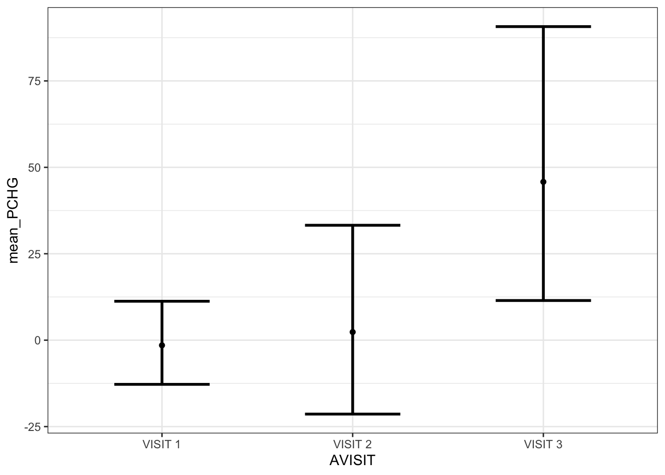
In this last final table, the geometric mean of the fold changes and the mean percent change, along with their 95% confidence intervals are shown. This should be the final desired picture of the estimates, with the p-values obtained in the above sections.
We can face some data in clinical trial work that is usually shown and analyzed in the log scale.
Change in the log transformed values is nothing but the logarithm of the fold changes. \(log(AVAL_{ij}) - log(BASE_i) = log(AVAL_{ij} / BASE_i)\)
If we exponentiate the mean of the log of the fold changes, we get our desired geometric mean of the fold changes.
When working with the log transformed fold changes, I demonstrated the Ho is still mean = 0, as the log(1) = 0 (1 means the fold change when there is null effect).
We have seen how the geometric mean of the fold changes can be converted to the mean percent change, in case there is a need for doing so.
With all this said, see you all in the next post! 🏀