Call:
lm(formula = hgt ~ splines::ns(age, knots = qts), data = mydata)

Residuals:
    Min      1Q  Median      3Q     Max
-33.641  -3.757   0.182   3.782  30.000

Coefficients:
                               Estimate Std. Error t value Pr(>|t|)
(Intercept)                     58.8252     0.2016   291.8   <2e-16 ***
splines::ns(age, knots = qts)1  70.6905     0.3936   179.6   <2e-16 ***
splines::ns(age, knots = qts)2 107.7958     0.3294   327.3   <2e-16 ***
splines::ns(age, knots = qts)3 177.5544     0.6570   270.3   <2e-16 ***
splines::ns(age, knots = qts)4  91.0141     0.5005   181.8   <2e-16 ***
---
Signif. codes:  0 '***' 0.001 '**' 0.01 '*' 0.05 '.' 0.1 ' ' 1

Residual standard error: 6.27 on 7298 degrees of freedom
Multiple R-squared:  0.9804,    Adjusted R-squared:  0.9804
F-statistic: 9.13e+04 on 4 and 7298 DF, p-value: < 2.2e-16Natural Cubic splines
Biostats
Introduction
In the past weeks I had an opportunity to deep dive on the standard reference growth charts provided by the Centers for Disease Control and Prevention (CDC), which are widely used by pediatricians and nurses to track the growth of infants, children and adolescents. I was interested in the LMS GAMLSS methodology used for getting the final reference centile curves. I first thought about spending some time of my past weekend to make a post around this topic as “knowledge sharing”. This LMS GAMLSS topic has a significant number of “black-box” dependencies to be understood though, and since I like demistyfying every piece that is behind the scenes of these models, I decided to start from the more simple basic dependencies so that we can keep building our knowledge on top of them.
This post is mainly focused on the Natural Cubic Splines.
Analysis data set
The complete sample of cross-sectional data from boys 0-21 years used to construct the Dutch growth references 1997 is going to be used for the analysis. The intent is to keep using this same data set in the future related posts as well. This data set is exported by the package AGD.
We will be focusing on modelling the height-age relationship.
Some basics
Ordinary Least Square Regression
I am pretty sure most of you are more than familiarized with the Linear Models plus it is not the scope of this post. This will help us connecting the later dots though.
Taking a look at the height vs age scatter plot above, the most simplistic (not the best) way would be to fit a straight line by a linear model by using a Ordinary Least Square Regression (OLS). In the OLS Regression Model we will be estimating the conditional expected means of our outcome as a linear combination of the predictors where each of them has a different effect (\(\beta_j\)) in the outcome. See (Equation 1)
\[ E(Y|X) = \beta_0 + \sum_{j = 1}^{m} \beta_jx_j + \epsilon \tag{1}\] Where:
- \(x_j\) are the different predictor variables.
- \(\beta_0\) is the coefficient corresponding to the intercept.
- \(\beta_j\) are the coefficients corresponding to the \(x_j\) covariates.
- \(\epsilon\) is the error term (variability not explained by the model).
The assumptions we are making when going over this Simple Linear Regressions are the following ones:
- There is a linear relationship between dependendant variable and the predictor.
- The difference (residuals) between the observed values \(y_i\)-s and their matching conditonal expected value (\(E[Y|X]\)) follows a normal distribution with mean 0 and and a standard deviation \(\sigma\) (\(\epsilon\_i\sim N(0,\sigma)\)).
- \(\sigma\) is constant across \(X\) (no \(i\) subscript in \(N(0,\sigma)\)) (homoscedasticity).
- Observations \(y_i\) are independent to each other.
In the next height vs age scatter plot where the OLS fitted line is superimposed, it clearly suggests the relationship is not linear across all age ranges.
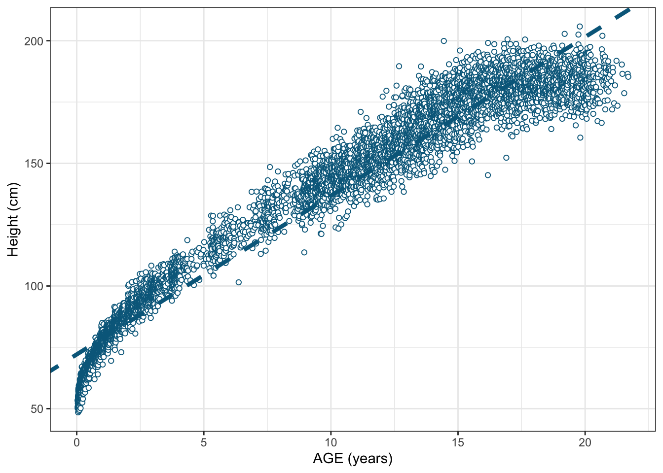
Let’s go beyond OLS then!
Generalized Linear Model
Instead of directly jumping from Ordinary Linear Regression to Generalized Additive Models (which is the main broad topic to be discussed in this post), let’s briefly talk about the Generalized Linear Models (GLM) term, which beautifully “links” (never better said) the OLS and GAM terms (GAM is part of GLM).
GLM is the flexible generalization of the OLS regression presented above. Rather than just modelling the expected value directly as a linear combination of the predictors, there is a link function relating the expected conditional value with the linear combination of the predictors (Equation 1).
- The conditional \(Y_i\) values do NOT need to be normally distributed, but it typically assumes conditional distributions coming from an exponential family (e.g binomial, Poisson, multinomial, normal, etc). General additive models for Location, Scale and Shape (GAMLSS) relax this assumption of exponential families by replacing by a general distribution family (skewed, kurtotic). This is actually the method to be used to estimate the final CDC growth charts, but we have still a lot of work to do before we reach this GAMLSS topic. If you want to go faster, check Rigby et al
- GLM does NOT assume a linear relationship between the response variable and the explanatory variables, but it does assume a linear relationship between the transformed expected response in terms of the link function and the explanatory variables (i.e the logit function at the logistic regression).
We can just enhance the (Equation 1) to get the generalized equation.
\[ ln[p/(1-p)] = \beta_0 + \sum_{j = 1}^{m} \beta_jx_j + \epsilon \tag{2}\]
Where: \(g(.)\) is the link function. For instance, in the OLS regression the link function is the identity link function, where (Equation 2) converts back into (Equation 1).
After this short introduction on GLM, we are more ready to talk about the General Additive Models (GAM).
Generalized additive models (GAM)
Coming back to the height vs age modelling, the OLS model could be extended to accommodate, for non-linear effects using some polynomials. However, sometimes it is quite hard to find the best polynomial equation that fits the data the best. Once said this… let’s give General Additive Models (GAM) a try!.
GAM models are no longer dependant on the linear combination of the predictors, but on the linear combination of unknown smooth functions of the predictors, keep this statement in mind. Saying this in a friendlier manner (and you will understand this as we go forward on the content), we will try modelling the height vs age relationship by linearly combining our new very simple “mini-polynomials”. Let’s make our new “mini-polynomial” friends work for us to achieve a more complex outcome.
\[ g(E(Y|X)) = \beta_0 + \sum_{j = 1}^{J} \beta_jf_j(x) + \epsilon \tag{3}\]
See \(f_j(x)\) from (Equation 3) who are our simpler polynomial smooth function friends who are actually called basis functions that are going to help us obtain the final spline curve, by their linear combination. Then we can say, the resulting spline is the sum of these weighted basis functions, evaluated at the values of \(x\) (age in our specific case). The predictor \(x\) can be a single variable or multiple variables. Our discussion will focus on a univariate function (age). Then \(j\) represents the different basis functions in (Equation 3).
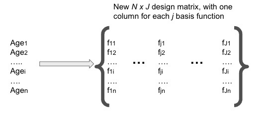
The only thing we are doing here is replacing the age variable by the basis functions \(f_j(x)\). From now on, consider these basis functions as independent covariates where they will have their own effect coefficient and place in the design matrix.
Presenting our basis function friends
Let me further introduce you these basis functions that are going to help us along this journey with the aim of improving the non so accurate linear height on age dependency obtained from the OLS model. But first of all, we will need to start partitioning the range of \(X\) (age) in a smaller intervals by adding knots, in order to solve the non-locality issue we may observe when fitting a global polynomial to the entire range of \(X\).
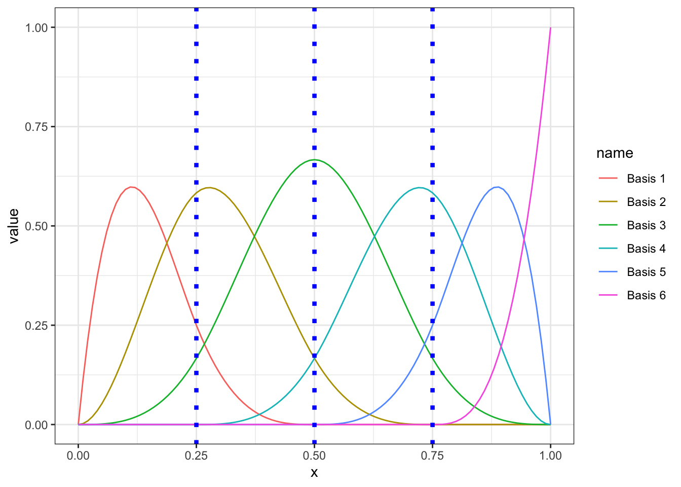
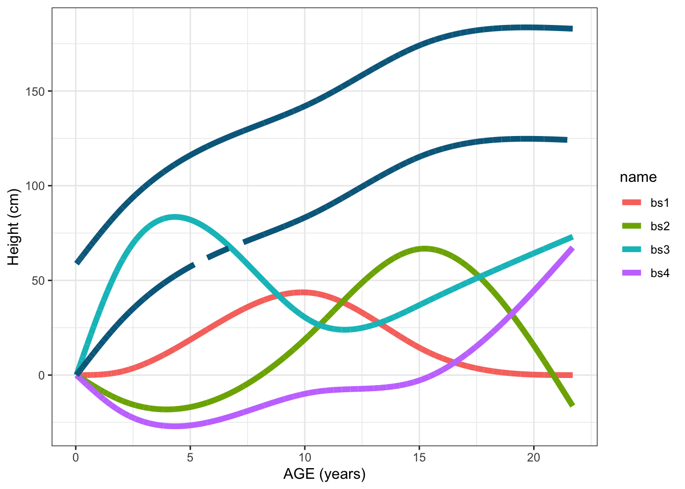
As an example, see the following basis function examples evaluated on a vector \(x\) (sequence from 0 to 1). Cubic polynomial basis functions will be used (d = 3), which are called B-splines (widely used). These are going to be piecewise cubic polynomial functions in between knots. I would recommend visiting 7.3 and 7.4 sections of An Introduction to Statistical Learning to further understand the relation between piecewise regression and the final splines. 3 knots (25%, 50% and 75% centiles) will be located in the following examples.
In Figure 3, all the effects (\(\beta_j\)-s from Equation 3) are set to 1. The number of B-splines or basis functions are defined by the number of knots (3) + the degrees of freedom of the basis functions (3), and this is why we are seeing 6 curves in the next figure. They can easily be obtained with splines::bs() function. The vertical blue dashed lines are the location of the three knots. You could try using splines::bs() with a different number and location of knots and going over the same plot.
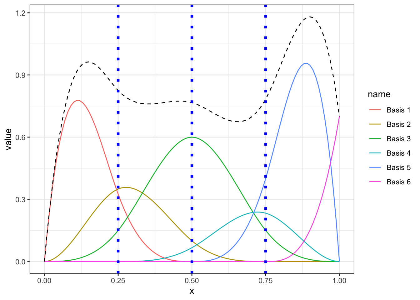
Similarly, In Figure 4, I am randomly assigning different effects to each of the 6 basis functions, meaning each of them will have different impact on the final resulting spline curve, which is presented as a black dashed line in the figure.
Fitting a natural cubic spline in our data
Now, we are going to try to make use of the cubic splines to model the height and age relationship. See some notes:
- We will force the basis splines to be linear at boundaries (2nd derivatives are zero at the boundaries). This makes the cubic B-splines to be turned into restricted or natural cubic splines. Looking at our height vs age scatter plot, it makes sense forcing linearity at boundaries. In this way, we will be reducing the number of basis splines from 6 to 4 (assuming 3 knots are used).
- The identity link function \(g(.)\) is used.
- In this post we are not going to focus on the selection of the optimal number of knots and the concept of penalized splines or smoothed splines (we will keep this for another later post). Let’s start from the simplest scenario where the location and the number of knots will be determined by us. Three different scenarios will be covered so that we can actually observe the impact of the number and the location of knots by fitting 3 independent natural cubic splines with 1, 3 and 5 knots.
In the following plot the three splines (by using 1, 3 and 5 knots) are shown along with the scatter plot and the OLS fitted line. Natural cubic splines can be easily fitted by the widely used lm() function. Keep in mind that, although we are now using the basis functions (evaluated on age) instead of the age, we are still modelling the height as a linear combination of these basis functions.
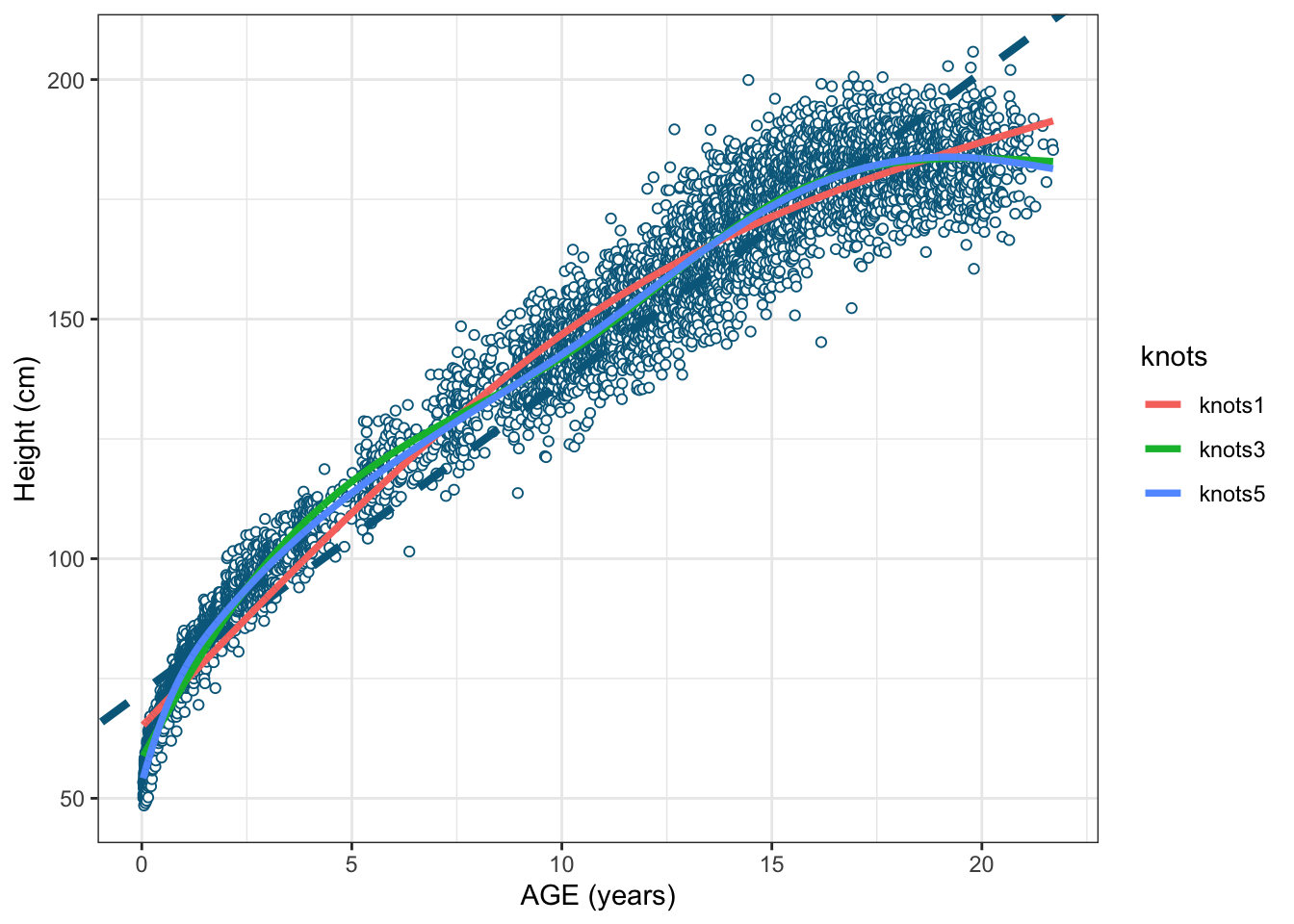
The adjusted R-squared values we get from the 3 natural cubic splines are 0.9729258, 0.9803982 and 0.9813835, for k = 1, k = 3, and k = 5 knots, respectively (model slightly improved by increasing knots). Just taking the model with 3 knots as an example, see the summary of the resulting spline model where the estimated coefficients \(\beta0\) (intercept), \(\beta1\), \(\beta2\), \(\beta3\) and \(\beta4\) corresponding to the four basis functions are shown.
How we can get the fitted line predictions manually?
It is always good to understand how these predicted values are obtained. See the two main elements.
- 5 x 1 \(\beta\) coefficient matrix column.
                   (Intercept) splines::ns(age, knots = qts)1
                      58.82522                       70.69047
splines::ns(age, knots = qts)2 splines::ns(age, knots = qts)3
                     107.79577                      177.55442
splines::ns(age, knots = qts)4
91.01409 - A 7303 row (number of observations) x 5 column design matrix where each column corresponds to the intercept and the 4 basis functions (model with 3 knots) evaluated on the age values.
  (Intercept) splines::ns(age, knots = qts)1 splines::ns(age, knots = qts)2
1           1                   0.000000e+00                   0.0000000000
2           1                   9.377398e-11                  -0.0002162559
3           1                   9.377398e-11                  -0.0002162559
4           1                   7.501918e-10                  -0.0004325114
5           1                   4.622710e-09                  -0.0007929355
6           1                   9.530215e-09                  -0.0010091882
  splines::ns(age, knots = qts)3 splines::ns(age, knots = qts)4
1                   0.0000000000                   0.0000000000
2                   0.0005867545                  -0.0003704986
3                   0.0005867545                  -0.0003704986
4                   0.0011735079                  -0.0007409965
5                   0.0021514254                  -0.0013584899
6                   0.0027381712                  -0.0017289830
By taking advantage of some basic matrix algebra and mathematical operations that sit behind linear regression, the design matrix corresponding to the 4 basis functions and the \(\beta\) coefficients are multiplied by using matrix multiplications \(\beta X\)
The result of the matrix multiplication \(\beta X\) provides the same line obtained as by using predict() function. In the next figure, the following lines are plotted:
- Each of the 4 basis functions multiplied by their corresponding coefficient \(\beta_j\) (\(j = 1, ... 4\))
- The predicted line (solid line) obtained by the matrix multiplication \(\beta X\) explained above.
- The dashed line which is the same matrix multiplication but excluding the intercept (this is why they are parallel lines) with the aim of seeing the only contribution of the basis functions.
Adding an additional covariate
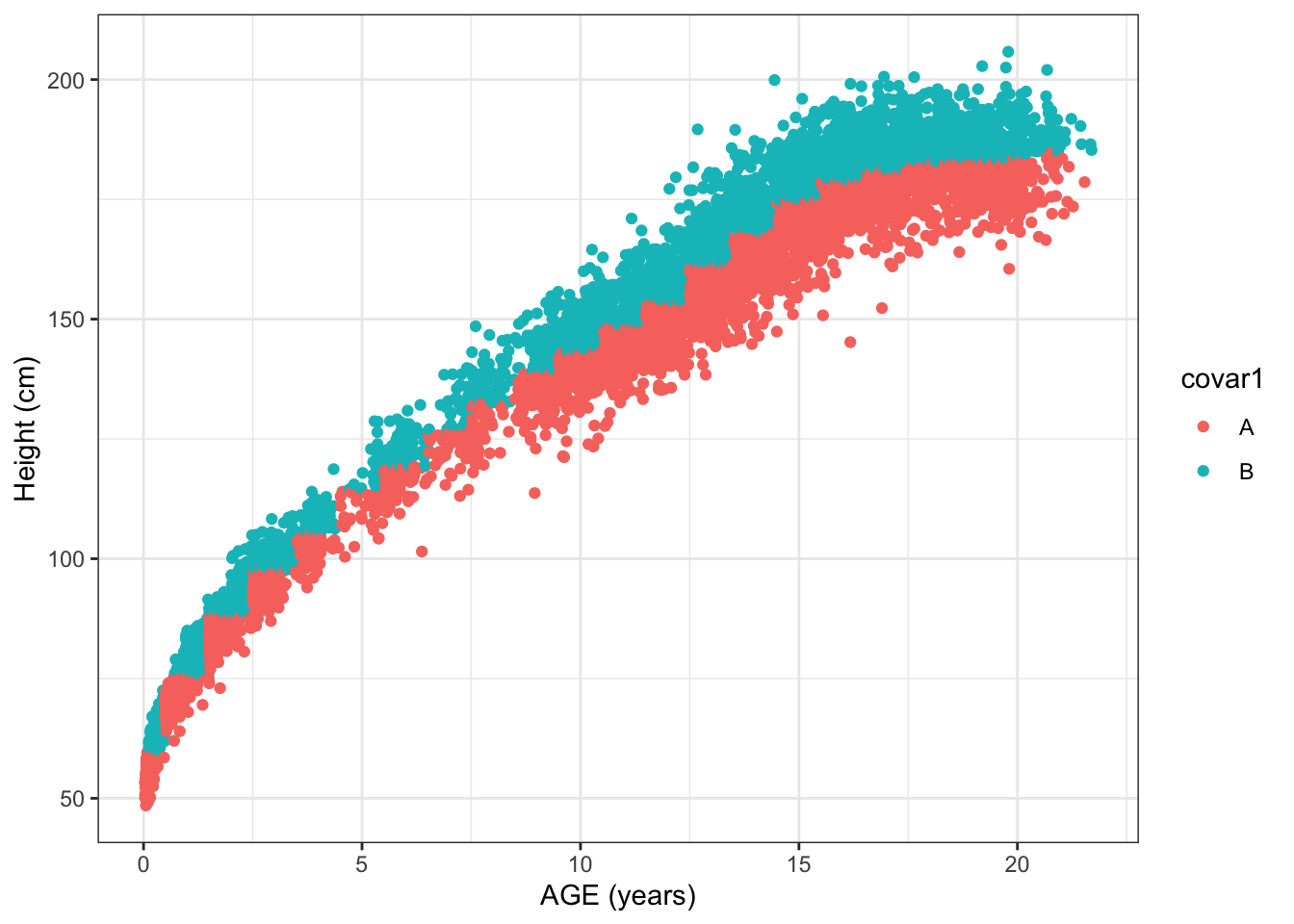
We can perfectly add an additional covariate(s) to the above model. For this example, I will create synthetic binary (A and B values) variable with a pronounced effect on height. The new equation for this specific case would be:
\[ \hat{y}_i = \hat{\beta_0} + \sum_{1}^{4} \hat{\beta_j}b_j(age_i) + \hat{\beta}_{j+1}Covar1 + \epsilon_i \tag{4}\]
This new covariate addition in the model will check whether there is any systematic shift on the height (marginal effect) between Covar1 levels.
Now the design matrix will contain an additional column corresponding to the new covariate in place in the model.
  (Intercept) splines::ns(age, knots = qt3)1 splines::ns(age, knots = qt3)2
1           1                   0.000000e+00                              0
2           1                   9.376466e-09                              0
3           1                   9.376466e-09                              0
4           1                   7.501173e-08                              0
5           1                   4.622251e-07                              0
6           1                   9.529268e-07                              0
  splines::ns(age, knots = qt3)3 splines::ns(age, knots = qt3)4
1                              0                   0.0000000000
2                              0                  -0.0009827484
3                              0                  -0.0009827484
4                              0                  -0.0019654206
5                              0                  -0.0036028316
6                              0                  -0.0045849284
  splines::ns(age, knots = qt3)5 splines::ns(age, knots = qt3)6 covar1B
1                    0.000000000                    0.000000000       0
2                    0.003577737                   -0.002594988       0
3                    0.003577737                   -0.002594988       0
4                    0.007155197                   -0.005189776       0
5                    0.013116260                   -0.009513428       0
6                    0.016691625                   -0.012106696       0
We can conclude there is an statistically significant effect of Covar1 as I made sure to introduce this additive effect on the model. With this example, I just wanted to show that we can still add other covariates in the context of splines.
Call:
lm(formula = hgt ~ splines::ns(age, knots = qt3) + covar1, data = mydata3)
Residuals:
Min 1Q Median 3Q Max
-28.9708 -2.9214 0.0392 2.8542 25.6663
Coefficients:
Estimate Std. Error t value Pr(>|t|)
(Intercept) 51.9506 0.2275 228.3 <2e-16 ***
splines::ns(age, knots = qt3)1 59.4407 0.4219 140.9 <2e-16 ***
splines::ns(age, knots = qt3)2 77.4694 0.4477 173.0 <2e-16 ***
splines::ns(age, knots = qt3)3 120.4993 0.3402 354.2 <2e-16 ***
splines::ns(age, knots = qt3)4 125.9757 0.3766 334.5 <2e-16 ***
splines::ns(age, knots = qt3)5 140.0315 0.6199 225.9 <2e-16 ***
splines::ns(age, knots = qt3)6 114.9681 0.6180 186.0 <2e-16 ***
covar1B 8.3631 0.1056 79.2 <2e-16 ***
---
Signif. codes: 0 '***' 0.001 '**' 0.01 '*' 0.05 '.' 0.1 ' ' 1
Residual standard error: 4.481 on 7295 degrees of freedom
Multiple R-squared: 0.99, Adjusted R-squared: 0.99
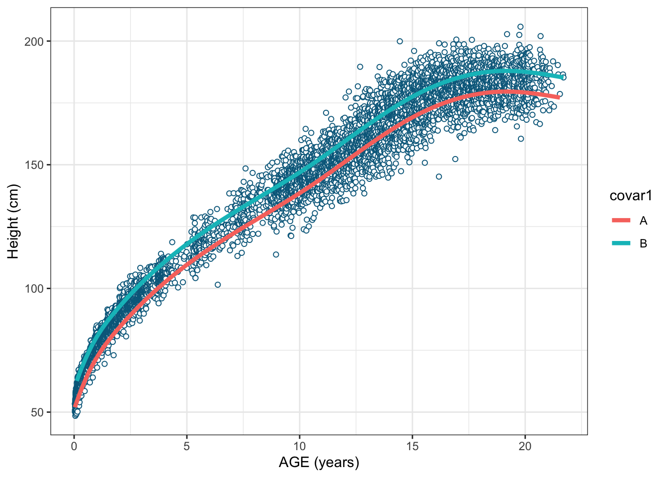
F-statistic: 1.032e+05 on 7 and 7295 DF, p-value: < 2.2e-16These new model could be visualized as two parallel lines (see figure 8) where the covariate Covar is introducing a systematic effect/increase in height across all age range when it takes value B.
Recap
After reading this, I hope you have a clearer understanding about the natural cubic splines and their use case when modelling non-linear trends. Often times we start using more complex models (i.e penalized splines, not covered in this post) without trying the simple ways such as the natural cubic splines presented in this post (they can perform as well as the penalized splines in some cases).
See the summary notes on what we have covered so far in this post:
- Quick refresh on the OLS model to start from the basics.
- GLM broader concept introduction to later present the GAM (subset of GLM).
- Concept of basis functions.
- Deep dive on the natural cubic splines which are the simplest GAM models (smoothed splines or penalized splines were not the scope of this post). Very important to understand the basics before working on more complex GAM models.
- The only relevant functions used so far in this post are lm(), ns() and bs()