Confidence Intervals for the Spearman Correlation Coefficient
Biostats
Author
Imanol Zubizarreta
Published
December 26, 2024
Introduction
In my field of work, data often do not meet the assumptions required for using Pearson’s Correlation Coefficient. As a result, Spearman’s correlation is frequently used as an alternative. Spearman’s correlation is a non-parametric measure of association based on the ranks of the data. It evaluates the strength and direction of the monotonic relationship between two variables. Addison et al is one of the many examples utilizing Spearman’s correlation coefficient to assess associations between different baseline biomarkers and their relationship with clinical outcomes of interest.
There are some R packages providing the 95% confidence intervals for the Spearman Correlation Coefficient. As biostatisticians, it is not enough to rely on software to churn out results; we must understand the principles behind the methodologies we use. Choosing the correct method requires a clear understanding of these principles to ensure that the results are both meaningful and appropriate for the data at hand.
Objective
In this post, I will compare two methods for computing confidence intervals for Spearman’s Correlation Coefficient using simulated data sets with varying sample sizes and correlation levels:
Fisher’s Z transformation that is supported by the DescTools::SpearmanRho function.
Jackknife Euclidean as well as Empirical likelihood-based inference methods that are supported by SpearmanCI::SpearmanCI function.
Simulated Data sets
1000 bivariate log-normal random samples were generated for each of the following scenarios:
sample size n = 20, 40, 60, 80, 100
Spearman target correlation coefficients of 0.2, 0.4, 0.6, 0.8
But, how to simulate bivariate log-normal data with a given Spearman Correlation Coefficient (not Pearson Correlation Coefficient)? See the steps followed for achieving this:
Generate a random bivariate normal samples with the desired Pearson correlation coefficient
Rank the data to match the Spearman correlation
Convert ranks to uniform. Spearman correlation is invariant under monotonic transformations. By mapping ranks to a uniform scale, you create a standardized space where further transformations can be applied.
Once the ranks are on a uniform [0, 1] scale, they can be mapped to any desired distribution such as lognormal, using the inverse cumulative distribution function (also called as the quantile function).
Finally calculate the sample Spearman correlation.
The two methods tested for calculating 95% Confidence Intervals
Fisher’s Z transformation
The Fisher’s Z transformation is a method for transforming the correlation coefficient to a normally distributed variable. The transformation is defined as \[f(r) = arctanh(r)\] where \(r\) is the correlation coefficient. DescTools::SpearmanRho function provides Fisher’s transformation based confidence intervals for Spearman correlation coefficient.
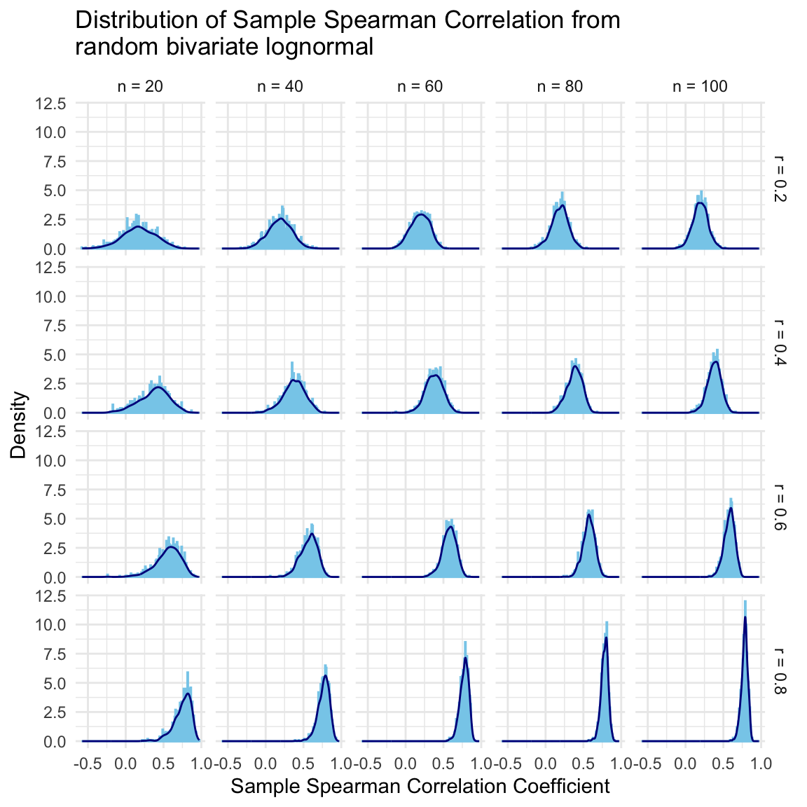
SAS documentation shows how Pearson’s correlation coefficient’s distributions are usually very skewed when the correlations are large in magnitude, and how Fisher’s transformation turn these distributions into normal distributions. Thereby, I wanted to confirm the same would be expected for Spearman’s correlation coefficient, to make sure we can assume normality of the distributions when calculating confidence intervals.
The following graph shows the sampling distribution of the Spearman correlation coefficients obtained in the simulations. It is pretty straightforward to see that distributions are skewed to the left mainly in the scenarios with large correlation coefficients and small number of observations. Variance and the skewness of the distributions depend on the underlying correlation coefficient and the sample size.
Code
ggplot(simulated_data, aes(x = spearman_cor)) +geom_histogram(aes(y =after_stat(density)), binwidth =0.01, color ="skyblue") +geom_density(color ="darkblue") +facet_grid(target_spearman_cor_label ~ n_label) +# Facet by group1 (rows) and group2 (columns)theme_minimal() +labs(title ="Distribution of Sample Spearman Correlation from\nrandom bivariate lognormal",x ="Sample Spearman Correlation Coefficient",y ="Density" )
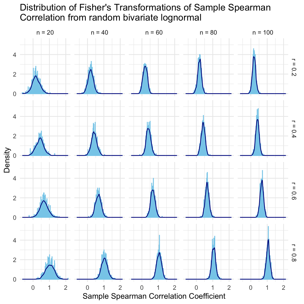
When applying the Fisher’s transformation, the distributions are pretty normal now and the variance is not dependant on the target correlation anymore (variance stabilizing transformation), which are good news! 😃 See the distributions for the Fisher’s transformed values.
Code
ggplot(simulated_data, aes(x =atanh(spearman_cor))) +geom_histogram(aes(y =after_stat(density)), binwidth =0.01, color ="skyblue") +geom_density(color ="darkblue") +facet_grid(target_spearman_cor_label ~ n_label) +# Facet by group1 (rows) and group2 (columns)theme_minimal() +labs(title ="Distribution of Fisher's Transformations of Sample Spearman\nCorrelation from random bivariate lognormal",x ="Sample Spearman Correlation Coefficient",y ="Density",fontsize =0.5 )
Ignoring unknown labels:
• fontsize : "0.5"
The final confidence interval for the correlation coefficient is obtained by back-transforming the confidence interval for the transformed variable. The 95% confidence intervals obtained in this way, will always lie entirely within the valid range of [-1, 1], and the upper bound will never exceed 1.
Jackknife Likelihood based method
This approach assumes the jackknife log-likelihood function of the Spearman parameter asymptotically converges to a Chi-square distribution of 1 degrees of freedom. Thereby, the bounds of the 95% confidence interval is constructed by the roots of the function \(-2L(\theta) - \chi^2_{1, 0.95}\), where \(L(\theta)\) is the log likelihood function and \(\chi^2_{1, 0.95}\) is the 95th quantile of the chi-square distribution with one degree of freedom.
SpearmanCI provides these confidence intervals and is based on the paper by de Carvalho et al. The package provides an option to use the Empirical as well as Euclidean likelihood.
Error message when using the Jackknife Euclidean likelihood method with small number of observations
SpearmanCI under the Euclidean method was often giving an error message when calculating the confidence intervals for the lowest simulated sample size (n = 20) and highest correlation level (r = 0.8). The following data frame shows the proportion (%) of cases that lead to an error out of 1000 simulations attempted for each correlation coefficient and sample size combination. See the high proportion of errors (~50%) faced when n = 20 under highly correlated data.
The error message I was getting was the following: Skipping calculation for n = 20.000000 and target correlation = 0.800000 due to error: f() values at end points not of opposite sign
See one of the simulated random bivariate log-normal data that lead to this error when using the Jackknife Euclidean likelihood approach:
As you can see in the following message, when making use of the spearmanCI function on the above data set with the Euclidean method, we are able to replicate the error message.
An error occurred:  f() values at end points not of opposite sign
Execution finished.
The root cause of the error is the following: The function cannot find the root for\(-2L(\theta) - \chi^2_{1, 0.95}\) between the Spearman Correlation Coefficient and the value of 1, when trying to get the upper limit of the 95% confidence interval. This happens when the correlation is high, and sample size is low.
I went deep on the body of this SpearmanCI function.
Code
x <- example_data_error$xy <- example_data_error$yU <-cor(x, y, method ="spearman") #Spearman correlation coefficientn <-length(x)Z <-as.double() #Jacknife pseudovaluesfor(i in1:n) Z[i] <- n * U - (n -1) *cor(x[-i], y[-i], method ="spearman")#function for the standard deviation of the pseudovaluess <-function(theta) 1/ n *sum((Z - theta)^2)#function for the likelihood - chisq quantile for alpha = 0.05 and degrees of freedom = 1g <-function(theta) n * (U - theta)^2/s(theta) -qchisq(0.95, 1)
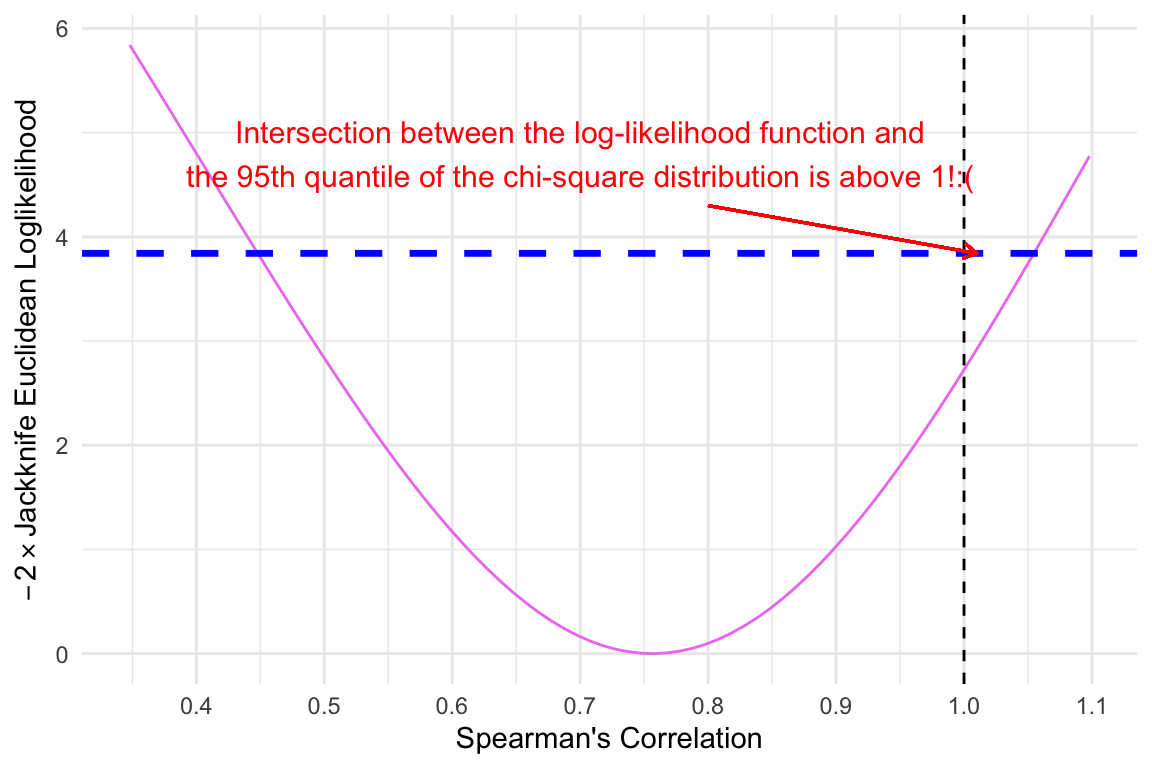
I replaced the interval [Spearman Estimate, 1]SpearmanCI uses to calculate the root of \(-2L(\theta) - \chi^2_{1, 0.95}\) and get the upper bound of the 95% confidence interval, by [Spearman Estimate, 1.1]. You can see the root found is above 1. This is why the Euclidean likelihood method of SpearmanCI results in an error.
Code
upper <-uniroot(g, interval =c(U, 1.1), tol = .1*10^{-10})$rootupper
[1] 1.000132
The dashed blue colored horizontal line is the Chi-square quantile for alpha = 0.05 and df = 1 and the violet colored curve is the log likelihood function. The visualization clearly shows that the upper intersection between the dashed line and the log-likelihood curve occurs above 1, which aligns with the root identified in the code chunk above.
Code
#l = the lower limit of the confidence intervall <-uniroot(g, interval =c(-1, U), tol = .1*10^{-10})$roottheta2 <-seq(l-0.1, 1.1, 0.01)likelihood2 <-sapply(theta2, FUN =function(theta2) {n * (U - theta2)^2/s(theta2)})plot_df2 <-data.frame(theta = theta2, likelihood = likelihood2)ggplot(plot_df2, aes(x = theta2, y = likelihood2)) +geom_line(color ="violet") +geom_hline(yintercept =qchisq(0.95, 1), linetype ="dashed", color ="blue", linewidth =1.2) +geom_vline(xintercept =1, linetype ="dashed") +xlab("Spearman's Correlation") +ylab(expression(paste(-2%*%"Jackknife Euclidean Loglikelihood"))) +geom_segment(aes(x =0.8, y =4.3, xend =1.01, yend =3.841459), # Arrow from (4, 10) to (4, 9)arrow =arrow(length =unit(0.2, "cm")), # Arrowhead sizecolor ="red" ) +annotate("text", x =0.7, y =4.8, label ="Intersection between the log-likelihood function and\nthe 95th quantile of the chi-square distribution is above 1!:(", size =4, color ="red" ) +theme_minimal() +scale_x_continuous(breaks =seq(0, 1.1, by =0.1))
Warning in geom_segment(aes(x = 0.8, y = 4.3, xend = 1.01, yend = 3.841459), : All aesthetics have length 1, but the data has 60 rows.
ℹ Please consider using `annotate()` or provide this layer with data containing
  a single row.
Upper bound of the 95% Confidence Interval is above 1 when using the Jackknife Empirical log likelihood method
As mentioned before, the SpearmanCI also provides an option to use the Empirical log likelihood approach. See the proportion of cases that lead to an upper bound of the 95% confidence interval > 1 out of 1000 simulations attempted for each correlation coefficient and sample size combination. Definitely not the outcome we would like to face when the correlation is high and the sample size is low!
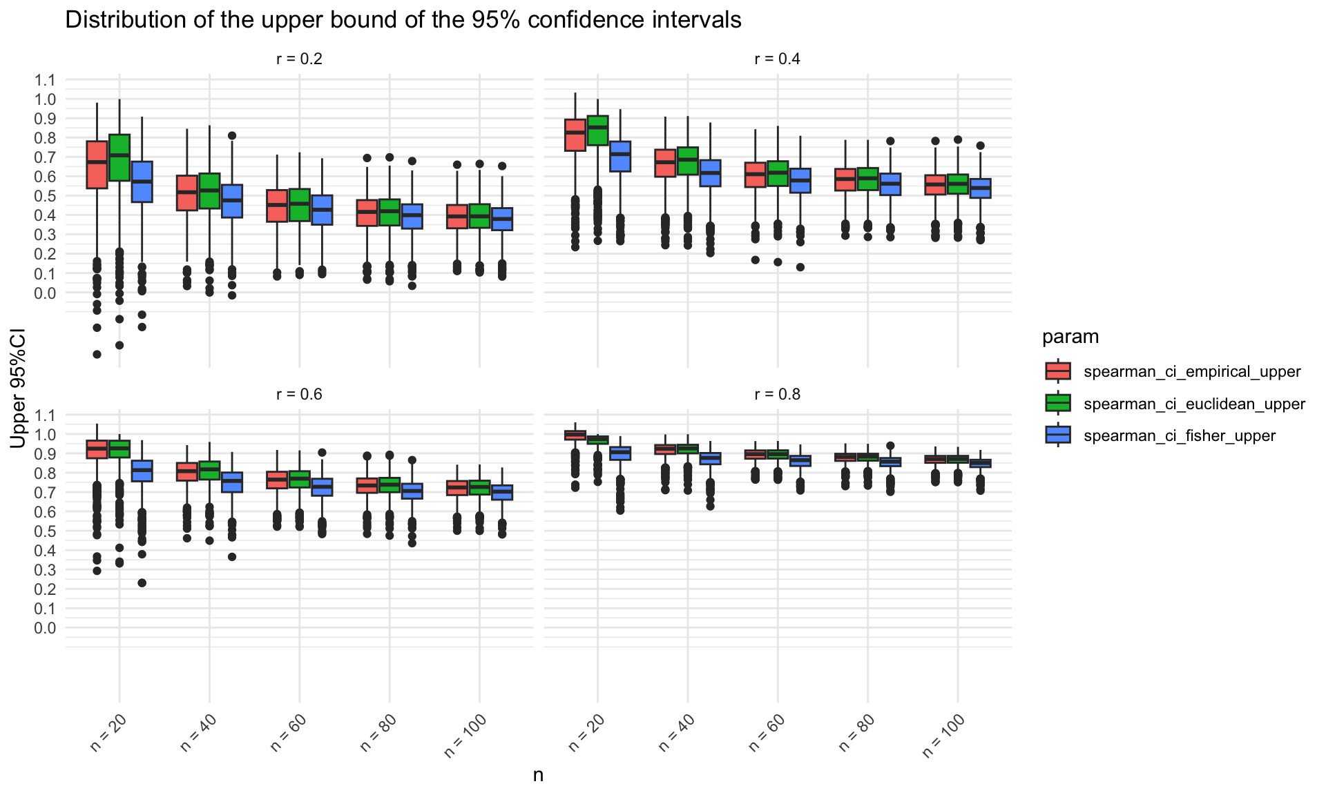
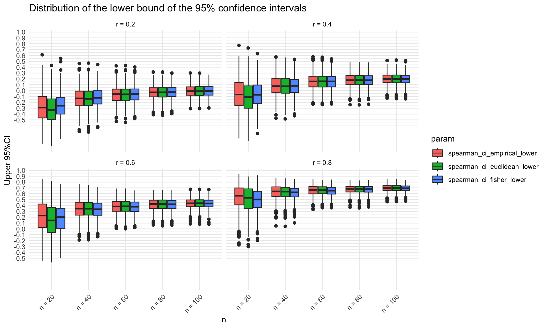
Distributions of the three type confidence intervals
In the following graphs, the distributions of the upper and lower limits of the 95% confidence intervals are shown by the use of the three methods. The upper bounds of the 95% confidence intervals obtained in the simulations are systematically higher when using the jackknife likelihood approach (either Euclidean or Empirical) compared to the bounds obtained by using the Fisher’s Z transformation. These differences are more pronounced for small sample sizes. The lower bounds of the 95% confidence intervals are pretty similar across methods. The opposite would happen with negatively correlated data, where the Jackknife likelihood approach would provide lower lower bounds of the confidence intervals and similar upper bounds.
Conclusion
See the main takeaways learnt in this post:
Fisher’s Z transformation is a good method for calculating confidence intervals for the Spearman correlation. The distributions of the transformed values are normal and the variance is not dependant on the target correlation anymore (variance stabilization). This is why we call The confidence intervals obtained will always lie entirely within the valid range of [-1, 1], and the upper bound will never exceed 1. Desctools::SpearmanRho function provides this method.
Jackknife likelihood method used by SpearmanCI::SpearmanCI is not suitable for small sample sizes and high correlation levels. Indeed, there is a reason we emphasized that that jackknife log-likelihood function of the Spearman parameter asymptotically converges to a Chi-square distribution of 1 degrees of freedom 😬. The Euclidean method SpearmanCI::SpearmanCI will often throw an error as the root of the function \(-2L(\theta) - \chi^2_{1, 0.95}\) is above 1, while the Empirical method will provide confidence intervals with upper bounds above 1, which is not desirable either.
The upper bounds of the 95% confidence intervals obtained in the simulations are systematically higher when using the jackknife likelihood approach (either Euclidean or Empirical) compared to the bounds obtained by using the Fisher’s Z transformation and these differences are more pronounced for small sample sizes.