Code
library(dplyr)
library(tidyr)
library(ggplot2)
library(mice)
library(ggExtra)library(dplyr)
library(tidyr)
library(ggplot2)
library(mice)
library(ggExtra)The main objectives of this post are:
Let me define a couple of functions that I will be systematically using throughout the post.
tidy_estimates_df <- function(df) {
  df %>%
    cbind(data.frame(param = c(
      "point_est", "se", "ci_lower", "ci_upper"
    ))) %>%
    as.data.frame() %>%
    tidyr::pivot_longer(
      cols = c("prop20", "prop40", "prop60", "prop80"),
      values_to = "Value",
      names_to = "missing_prop"
    ) %>%
    pivot_wider(id_cols = "missing_prop",
                values_from = "Value",
                names_from = "param")
}

plot_estimates <- function(df,
                           title = "Point estimates by starting missing proportion",
                           xlab = "Starting missing proportion (pre-imputation)",
                           ylab = "Point estimate and 95%CI",
                           imputations = FALSE,
                           group = NULL,
                           type_marginal = "density") {
  p1 <- ggplot2::ggplot(df,
                        aes_string(
                          x = ifelse(imputations, "imp", "missing_prop"),
                          y = "point_est",
                          group = group,
                          col = group
                        )) +
    geom_point() +
    theme_bw() +
    geom_errorbar(
      aes_string(ymin = "ci_lower", ymax = "ci_upper"),
      width = .1,
      linetype = 1
    ) +
    labs(title = title, x = xlab, y = ylab)

  if (imputations) {
    p1 <- ggMarginal(
      p1 + theme(axis.text.x = element_text(
        angle = 90,
        vjust = 0.5,
        hjust = 1,
        size = 5
      )),
      margins = "y",
      groupColour = TRUE,
      groupFill = TRUE,
      type = type_marginal
    )
  }

  p1
}The three variables of our analysis data sets are the following ones:
The following list of length 4 contains the data sets with different proportion of missingness (20, 40, 60, 80%) in the OUT variable that we generated here.
amp_df_list <- readRDS("../stats_ampute/amp_missing_df_list.rds")
names(amp_df_list) <- c(paste0("prop", c(20, 40, 60, 80)))
#head of the data set with 40% of missing
head(amp_df_list$prop40)
AGE OUT SUBJID
1 34.39524 74.58236 SUBJ-1
2 37.69823 100.53412 SUBJ-2
3 55.58708 NA SUBJ-3
4 40.70508 94.45932 SUBJ-4
5 41.29288 83.55338 SUBJ-5
6 57.15065 NA SUBJ-6Similarly, we have the starting complete data set.
df_complete <- readRDS("../stats_ampute/amp_starting_complete_df.rds")
head(df_complete)
SUBJID AGE OUT
1 SUBJ-1 34.39524 74.58236
2 SUBJ-2 37.69823 100.53412
3 SUBJ-3 55.58708 126.24033
4 SUBJ-4 40.70508 94.45932
5 SUBJ-5 41.29288 83.55338
6 SUBJ-6 57.15065 133.40075In the clinical trial setting you may have longitudinal data, and you may certainly be willing to estimate the difference in the outcome (i.e Change from baseline) between different treatment groups in an specific time point. However, a very simple point estimate is good enough to acquire this knowledge. The slope’s coefficient of the linear regression OUT ~ AGE will be the point estimate in this post. A point estimate by using the completed data set will be obtained in the following chunk of code. This will be our true/reference estimate for the later steps. We simulated the starting data set under the alternative hypothesis where there is an statistically significant age effect in the OUT variable under a significance level of alpha = 0.05.
Let’s get the true point estimate we would have obtained in the absence of missing data.
fit_true <- lm(OUT ~ AGE, data = df_complete)
fit_true_ci <- janitor::round_half_up(confint(fit_true, "AGE", 0.95), 3)
summary_fit_true <- summary(fit_true)
coef_true <- summary_fit_true$coefficients[2, 1]
se_true <- summary_fit_true$coefficients[2, 2]
fit_true_df <- data.frame(
  missing_prop = "Complete",
  point_est = coef_true,
  "se" = se_true,
  "ci_lower" = fit_true_ci[1],
  "ci_upper" = fit_true_ci[2]
  )
fit_true_df
missing_prop point_est se ci_lower ci_upper
1 Complete 2.062202 0.3083317 1.442 2.682The point estimate and the corresponding standard error are 2.0622024 and 0.3083317, respectively. It is up to you reducing/increasing the standard error by tweaking the OUT ~ AGE correlation when simulating the data 🙂.
Before talking about the multiple imputation and its associated between sample variance that I am willing to showcase in this post, worth first mentioning the non desired methodologies to handle missing data when missing data is under MAR condition, which is the condition under which we simulated missingness. Keep in mind the following anticipated statement before we go into the non-desired methodologies: The standard error of the point estimate obtained from the imputed data set, should not be lower than the original complete data set. Also, no need to highlight the point estimate should be unbiased.
Taking a look at the next table and figure (complete row contains the true estimates), we can conclude the single mean imputation (under MAR missingness) can have a negative impact when it comes to statistical inference. As the missing proportion increases, and under the simulated alternative hypothesis (AGE has an effect in the outcome):
Under MCAR, the mean imputation may not unbias the estimate, but it is not a condition we can assume many times in the field I work, as missingness and thereby the non-observed values potentially depend on other variables (i.e in clinical trials assuming the missing outcome can depend on the baseline characteristics added as covariates in the model, which would be the MAR assumption) or even on the variable itself.
results_mean_imp <- sapply(amp_df_list, FUN = function(amp_df) {
  amp_df <- amp_df %>%
    select(-SUBJID)
  #showing you can also go over the single mean imputations by using mice
  #you can get the complete data sets by using mice::complete()
  imp_df <- complete(mice::mice(amp_df, method = "mean", m = 1, maxit = 1, printFlag = FALSE))
  fit_imp_mean <- lm(OUT ~ AGE, data = imp_df)
  summary_fit_imp_mean <- summary(fit_imp_mean)
  ci <- janitor::round_half_up(confint(fit_imp_mean, 'AGE', level=0.95), 3)
  c("point_est" = summary_fit_imp_mean$coefficients[2, 1],
    "se" = summary_fit_imp_mean$coefficients[2, 2],
    "ci_lower" = ci[1],
    "ci_upper" = ci[2]
    )
}) %>%
  #making use the function defined at the top of the post
  tidy_estimates_df()

results_mean_imp <- fit_true_df  %>%
  rbind(results_mean_imp)


DT::datatable(results_mean_imp) #making use the function defined at the top of the post
plot_estimates(results_mean_imp)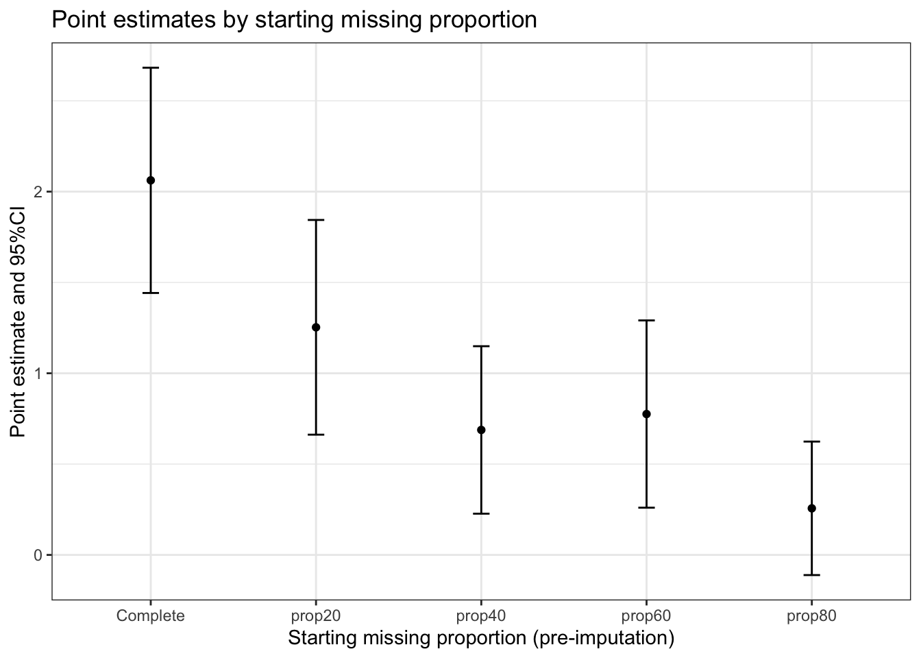
As shown in the previous section, we may have a hard time if we use single imputation methods (can be either mean, median, linear regression) to handle missing data under MAR due to a potential bias as well as the underestimation of the standard error (precision). This is when we start talking about the Multiple Imputation and the Between-sample variance which is the main topic I would like to highlight in this post.
Donald B. Rubin (1) observed that imputing one value (single imputation) for the missing value could not be correct in general, and this is when he started thinking about creating multiple imputations to be able to reflect uncertainty of the missing data. The three main steps (imputation + analysis + pooling) that compose the multiple imputation procedure are explained in the following sections. The following figure taken from van Buuren (2) describes the process.
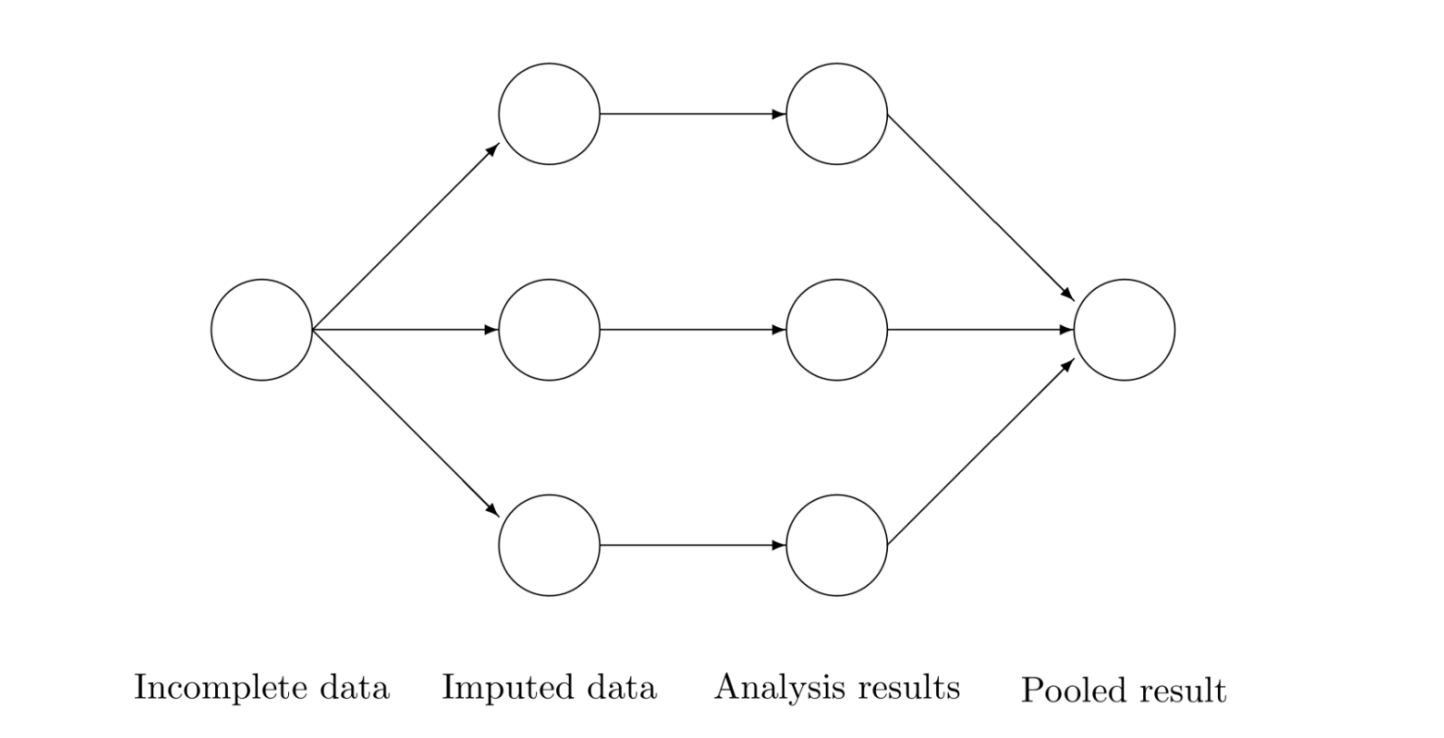
mice::mice() function will be used for this process.
We will create m = 100 number of imputed data sets by the chosen imputation model, leading to 100 number of complete data sets. In this post we will creating a high number of imputed data sets so that the later between-sample distributions can be more beautifully visualized in the later sections.
See some of the key parameters in the mice::mice function.
predictor_matrix <- matrix(c(0, 0,
                             1, 0)
                           , nrow = 2, byrow = TRUE)

colnames(predictor_matrix) <- c("AGE", "OUT")

rownames(predictor_matrix) <- c("AGE", "OUT")
Let’s go over the first step of generating 100 imputed data sets per missing proportion under analysis.
amp_df_list_no_subj <- lapply(amp_df_list, FUN = function(mylist) {
  mylist %>% select(-SUBJID)
})
imp_list <- lapply(amp_df_list_no_subj, FUN = function(df) {
 mice::mice(df, m = 100, predictorMatrix = predictor_matrix, method = "norm", print = FALSE)
})
mice::mice creates an object of class mids.
class(imp_list$prop20)[1] "mids"Please take a look at the other elements returned by the mids object. For instance, you can see the imputation equations that have been used so that you can make sure mice has been gone over your desired approach.
imp_list$prop20$formulas$AGE
AGE ~ `0`
<environment: 0x123fc6488>
$OUT
OUT ~ AGE
<environment: 0x123fc6488>You can also confirm you have been introducing the predictor matrix correctly:
imp_list$prop20$predictorMatrix AGE OUT
AGE 0 0
OUT 1 0In the next chunk of code we will be applying our target analysis model to each of the imputed data sets obtaining as many point estimates as imputed data sets (100 per missing proportion under analysis in our specific example). See the estimates of one of the regressions out of 400 we are generating.
imp_analysis_list <- lapply(imp_list, FUN = function(imp_dfs) {
  analysis <- with(imp_dfs, lm(OUT ~ AGE))
})

#showing one lm result out of 400 we generated
summary(imp_analysis_list$prop20$analyses[[1]])
Call:
lm(formula = OUT ~ AGE)

Residuals:
    Min      1Q  Median      3Q     Max
-35.398 -11.260  -0.965  11.285  47.748

Coefficients:
            Estimate Std. Error t value Pr(>|t|)
(Intercept)   5.1986    11.2050   0.464    0.645
AGE           2.1894     0.2708   8.084 1.64e-10 ***
---
Signif. codes:  0 '***' 0.001 '**' 0.01 '*' 0.05 '.' 0.1 ' ' 1

Residual standard error: 17.55 on 48 degrees of freedom
Multiple R-squared:  0.5765,    Adjusted R-squared:  0.5677
F-statistic: 65.35 on 1 and 48 DF, p-value: 1.644e-10Finally we pool/combine the by missing proportion specific m repeated complete-data point estimates (coefficients indicating the effect of age in the outcome) and variances. In this way we will have the average coefficient as the final effect, and the total variance that will account for the uncertainty due to missing data.
#Here we are getting the parameters such as the pooled estimates, within and between sample variances.
pooled_estimates_list <- lapply(imp_analysis_list, FUN = function(imp_analysis) {
 mice::pool(imp_analysis)
})

#rerunning this to get the confidence intervals
pooled_estimates_list_ci <- lapply(imp_analysis_list, FUN = function(imp_analysis) {
 summary(mice::pool(imp_analysis), conf.int = TRUE)
})

#see the pooled results
pooled_estimates_list_ci
$prop20
term estimate std.error statistic df p.value 2.5 %
1 (Intercept) -3.036051 14.4040900 -0.210777 28.03744 8.345857e-01 -32.539717
2 AGE 2.451411 0.3696576 6.631574 24.62130 6.476819e-07 1.689493
97.5 % conf.low conf.high
1 26.46762 -32.539717 26.46762
2 3.21333 1.689493 3.21333
$prop40
term estimate std.error statistic df p.value 2.5 %
1 (Intercept) 14.88822 16.0495133 0.9276432 19.37665 0.3650044586 -18.659655
2 AGE 1.88491 0.4344129 4.3389824 15.37839 0.0005532516 0.960961
97.5 % conf.low conf.high
1 48.436100 -18.659655 48.436100
2 2.808859 0.960961 2.808859
$prop60
term estimate std.error statistic df p.value 2.5 %
1 (Intercept) -16.655542 18.8853776 -0.8819279 17.64319 3.896733e-01 -56.38984
2 AGE 2.801569 0.5170205 5.4186804 13.72347 9.705936e-05 1.69057
97.5 % conf.low conf.high
1 23.078758 -56.38984 23.078758
2 3.912567 1.69057 3.912567
$prop80
term estimate std.error statistic df p.value 2.5 %
1 (Intercept) -7.124244 56.178643 -0.1268141 5.709579 0.9034348 -146.301277
2 AGE 2.920568 1.685693 1.7325618 3.751046 0.1629429 -1.884754
97.5 % conf.low conf.high
1 132.052790 -146.301277 132.052790
2 7.725889 -1.884754 7.725889For the confidence interval calculation of the pooled estimates, I would recommend going over the sections 9.3, 9.4 and 9.5 sections from the Applied Missing Data analysis with SPSS and R book (3).
Looking at the list above and the plot below, we can highlight the following:
#tidying the above list
results_mi <- fit_true_df %>%
  bind_rows(do.call(rbind, pooled_estimates_list_ci) %>%
  filter(term == "AGE") %>%
  select(point_est = estimate, se = std.error, ci_lower = `2.5 %`, ci_upper = `97.5 %`) %>%
bind_cols(missing_prop = c("prop20", "prop40", "prop60", "prop80")))#using the function defined in the beginning of the report.
plot_estimates(results_mi)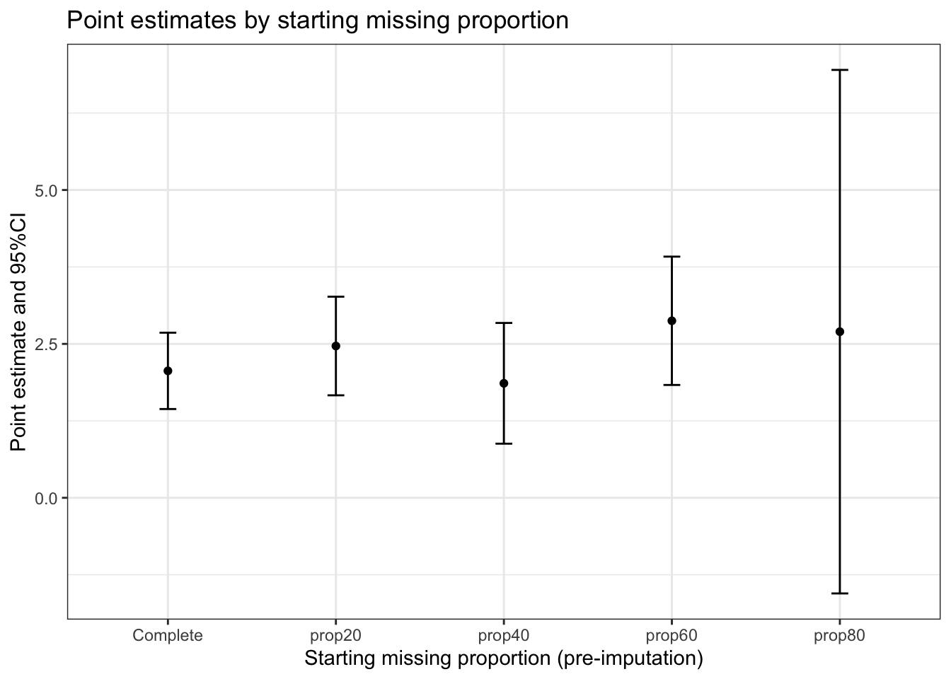
Explaining total variance calculation in the multiple imputation process is my ultimate goal in this post.
For this aim, demistifying the equation 2.17 from section 2.3 from Van Buuren’s book (2) by the use of some visualizations can be a good idea.
\[ V(Q|Y_{obs}) = \color{green}{E[V(Q|Y_{obs}, Y_{mis})|Y_{obs}]} + \color{red}{V(E(Q|Y_{obs}, Y_{mis})|Y_{obs})} = \color{green}{WithinSample} + \color{red}{BetweensSample} \]
The between sample variance B shows the closeness of agreement between each imputed-complete individual point estimate (coefficient indicating the effect of age in the outcome) and the combined/pooled final point estimate that the MI process provides. You will see that the following equation is nothing but the well-known equation for calculating the sample variance. This is exactly the piece of the total variance that accounts for the uncertainty due to missing data. Single imputation basically ignore this important point! 🤦🏽♂️
\[ B = {1/(m - 1)}\sum_{j = 1}^{m} (est_j - \overline{est})^2 \] Where \(\overline{est}\) is the pooled average point estimate and m the number of imputed data sets. For instance, we obtained a between-sample variance of 2.5770797 in the MI process applied to a data set with 80% of the outcome values missing, as shown under the b term.
pooled_estimates_list$prop80[2, ]Class: mipo m = NA
term m estimate ubar b t dfcom df riv
2 AGE 100 2.920568 0.2387114 2.57708 2.841562 48 3.751046 10.90376
lambda fmi
2 0.9159929 0.94088You can see that calculating the variance of the 100 individual point estimates yields the same exact result we have above under the b term (between sample variance)! 🥇
sapply(imp_analysis_list$prop80$analyses, FUN = function(estimates_tmp) {
  estimates_tmp$coefficients[2]
}) %>%
  var()
[1] 2.57708See the following figure with all the individual point estimates obtained from each of the imputed data sets, color coded by the starting missing proportion (100 imputed data sets for each missing proportion under analysis) along with the corresponding density plots. The dispersion/variation we see between the point estimates (within color) is exactly what the between-sample variance explains. As we concluded above, this uncertainty due to missing increases as the bigger is the starting missing proportion, as expected.
# Get the point estimate, standard error and confidence intervals.
imp_estimates_list <- lapply(names(imp_analysis_list), FUN = function(miss_prop_tmp) {
  analysis_list <- imp_analysis_list[[miss_prop_tmp]]
  analysis_list <- analysis_list$analyses
  do.call(rbind, sapply(analysis_list, FUN = function(analysis_tmp) {
  summary_fit_tmp <- summary(analysis_tmp)
  ci <- janitor::round_half_up(confint(analysis_tmp, 'AGE', level=0.95), 3)
  list(c("point_est" = summary_fit_tmp$coefficients[2, 1],
    "se" = summary_fit_tmp$coefficients[2, 2],
    "ci_lower" = ci[1],
    "ci_upper" = ci[2]
    ))
  })) %>%
    bind_cols(data.frame(miss_prop = rep(miss_prop_tmp, 100),
                         imp = paste0("imp", seq(1, 100)))) %>%
    mutate(imp = factor(imp, levels = paste0("imp", seq(1, 100))))
})


imp_estimates_df <- do.call(rbind, imp_estimates_list)

plot_estimates(
    df = imp_estimates_df,
    title = "Point estimates and 95%CI by missing proportion",
    imputations = TRUE,
    group = "miss_prop",
    type = "density",
    xlab = "1 to 100 imputed data sets")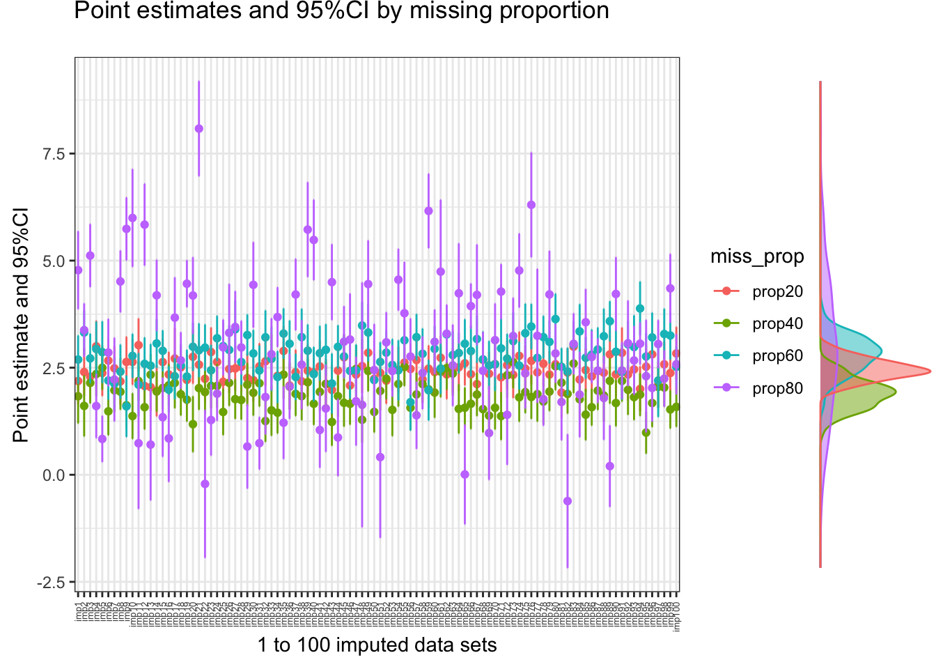
The within sample variance is nothing but the average of the repeated complete-data posterior variances of the point estimate. For instance, for the 80% of missing proportion case, we are getting the within sample variance of 0.2387114. In the following code chunk we are trying to get the same value by obtaining the individual estimate uncertainty values and calculating the average. Again, we are able to get the same exact value. 🤛🏽
sapply(imp_analysis_list$prop80$analyses, FUN = function(estimates_tmp) {
  summary_tmp <- summary(estimates_tmp)
  summary_tmp$coefficients[2,2]^2
}) %>%
  mean()
[1] 0.2387114When the number m of multiply imputed data sets is quite low, we need to consider the additional third between sample variance / m term to account for the low number of imputed data sets used for getting the pooled point estimate. By default, mice uses an m of 5, but we have been using an m of 100. Section 2.8 fron van Buuren (2) talks about the optimal number of multiply imputed data sets to be created.
These are the main topics we have covered so far in this post.
I spent some time of my long flight to San Francisco to work on this post. Cannot wait to meet my colleagues from Denali Therapeutics in person again! Exciting as well as intense week ahead. Let’s get it!
Picture taken from Mount Tamalpais.