| Subgroup | % of population | New drug | Placebo | Odds ratio |
|---|---|---|---|---|
| Biomarker positive | 50% | 80.0% | 33.3% | 8.0 |
| Biomarker negative | 50% | 25.0% | 4.0% | 8.0 |
| Combined | 100% | 52.5% | 18.7% | 4.8 |
Marginal vs conditional odds ratios: adjusting does not decide which one you get
Biostats
Estimands
Introduction
A while ago I came across a very interesting FDA statistical review of a trial with a binary endpoint. The applicant had fitted a GEE model, and the reviewer recommended a logistic generalized linear mixed model as a supplementary analysis. The applicant did it, and the review records the following.
The Applicant noted that the generalized linear mixed model is a conditional model with a subject-specific interpretation in contrast to the GEE model with a population average interpretation.
Two models, two odds ratios, and one of them is conditional while the other is population average. That is the topic of this post. I still see this distinction cause confusion, so I have tried to explain it with simple examples and visuals. Do not worry about the GEE and mixed model terminology as they are not needed to follow this post.
The study from that review has repeated visits and missing data. We stay with a single visit and complete data in this post 🙂.
FDA’s guidance on covariate adjustment makes the point in its Table 1. In a logistic model the covariate-adjusted odds ratio and the population-level odds ratio are different numbers, even under randomization and with a large sample. This is non-collapsibility, introduced briefly in the previous post.
Both numbers are correct, which is why the choice has to be made in advance. Sponsors “should specify whether the treatment effect of interest in an analysis is a conditional or unconditional treatment effect” (FDA, May 2023).
Two choices get mixed up here:
- Unadjusted or adjusted is about the model. Do we put covariates in it?
- Marginal or conditional is about the estimand. Which number are we trying to estimate? In a linear model the two are the same, so if you have only worked with continuous endpoints you may still be not familiarized with this concept 🤓
We can adjust for covariates and still target a marginal estimand, and we will see it in this post.
In this post we simulate a two-arm trial (1:1 allocation, arms called Active and Control) and estimate the treatment effect three ways from the same data: unadjusted, adjusted conditional, and adjusted marginal (g-computation). We watch what happens as the baseline covariate becomes more prognostic, then break the randomization and watch what changes. We will only focus on the point estimates in this post, so no confidence intervals and no standard errors here 🙂
The model and the two estimands
The data are generated from a logistic model with a single continuous prognostic covariate, BASE:
\[ \text{logit}\,P(Y = 1) = \alpha + \beta \cdot \text{TRT} + \gamma \cdot \text{BASE} \]
BASE is drawn from a standard normal distribution, so one unit is one standard deviation. The three parameters:
- \(\alpha\) is the intercept. It is solved numerically so the control-arm response rate is 30%.
- \(\beta\) is the treatment log-odds, fixed at \(\log(2.5)\) in every scenario.
- \(\gamma\) is the
BASElog-odds per standard deviation. This is the only quantity we vary, from \(\log(1)\) to \(\log(5)\). We move \(\gamma\) and show how far apart the conditional and the marginal odds ratio end up asBASEbecomes more prognostic.
This model has two true treatment effects, and they have different status.
- The conditional OR is \(\exp(\beta)\). We choose it when we write the model down, and it is 2.5 in everything that follows. It is the effect of treatment for patients who share the same value of
BASE. - The marginal OR is the odds ratio you get after predicting every patient’s risk under both arms and averaging those risks over the population. It is not a free parameter, because it follows from \(\alpha\), \(\beta\), \(\gamma\) and the distribution of
BASE.
Writing the marginal risk out for one arm makes the second bullet concrete. Let \(t = 1\) for Active and \(t = 0\) for Control, let \(\phi\) be the standard normal density, and let \(\text{expit}\) be the inverse of the logit, \(\text{expit}(x) = 1/(1+e^{-x})\), which turns a log-odds back into a probability. The true marginal risk integrates over the whole distribution of BASE:
\[ \bar p_t = \int \text{expit}\!\left(\alpha + \beta t + \gamma \cdot \text{BASE}\right)\phi(\text{BASE})\,\mathrm{d}\,\text{BASE} \]
G-computation, also called standardization, is the empirical version of that integral. It swaps the distribution for the patients actually in the trial, and the parameters for their estimates:
\[ \hat{\bar p}_t = \frac{1}{n}\sum_{i=1}^{n} \text{expit}\!\left(\hat\alpha + \hat\beta t + \hat\gamma \cdot \text{BASE}_i\right) \]
This is a counterfactual calculation. The sum runs over every patient in the trial, each one predicted under both arms, including the arm they were not given. The marginal odds ratio is then formed from \(\bar p_1\) and \(\bar p_0\) in the usual way.
Do not worry about the equations, you can even skip them 🙂 It is not rocket science: the FDA guidance on covariate adjustment describes the same calculation in six simple steps (FDA, May 2023, p. 7).
Simulated data
Everything below comes from simulated trials of 600 patients, 1:1 allocation, one visit, no missing data. Every number plotted later is the mean across 500 simulated trials.
| Scenario | BASE odds ratio per SD | Control-arm response rate | True conditional OR | True marginal OR |
|---|---|---|---|---|
| not prognostic | 1.00 | 30% | 2.500 | 2.500 |
| weakly prognostic | 1.50 | 30% | 2.500 | 2.418 |
| moderately prognostic | 2.50 | 30% | 2.500 | 2.185 |
| strongly prognostic | 5.00 | 30% | 2.500 | 1.885 |
The two agree only when BASE does “nothing”, i.e, when the baseline value is not a prognostic factor. As soon as the covariate predicts the outcome, the marginal OR is closer to 1 than the conditional one. That is non-collapsibility, and there is no confounding anywhere in this model.
What marginalizing does when BASE is prognostic
Every patient in this model has the same odds ratio. That is what conditioning on BASE means.
The animation below draws the two response curves, with BASE covariate on the horizontal axis, and walks along BASE from three standard deviations below the mean to three above. The dotted lines are the average risk in each arm, which is what marginalizing produces. The animation is inspired by Figure 1a of Daniel, Zhang and Farewell (Biometrical Journal 2021;63:528-557).
This section uses the moderately prognostic BASE scenario row of the table above. That choice is what makes the picture interesting. If BASE were not prognostic, the conditional and the marginal odds ratio would be the same number and there would be nothing to show.
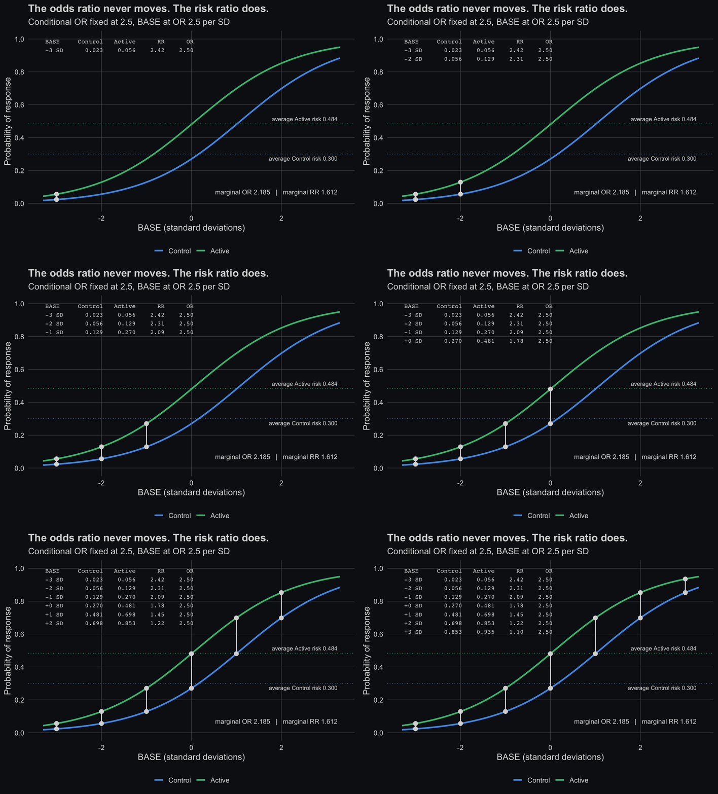
Three things to highlight:
- The odds ratio column never moves. The risk ratio column does. The risk ratio is 2.42 at three standard deviations below the mean of
BASE, 1.78 at the mean, and 1.10 three above. A risk ratio is not a single number unlessBASEis held fixed or the risks are marginalized. - The risk ratio is closest to the odds ratio where the response rate is lowest. At three standard deviations below the mean of
BASEthe control risk is 2% and the risk ratio is 2.42 against an odds ratio of 2.50. That is the rare-outcome agreement from the previous post. - The marginal odds ratio is closer to 1 than the conditional one. It is 2.18 against 2.50.
Jensen’s inequality
This is Jensen’s inequality: the average of a non-linear function is not the function evaluated at the average,
\[ E\!\left[g(X)\right] \neq g\!\left(E[X]\right). \]
It has one practical consequence worth stating. Setting BASE to its mean and reading the odds ratio out of the model returns \(\exp(\beta) = 2.5\). That is the conditional OR exactly, not an approximation to the marginal one.
With an identity link the average of the predictions equals the prediction at the average patient, and the two estimands are the same number. That is why the question does not arise for a continuous endpoint analyzed with ANCOVA or MMRM! 😬
Three estimators
We fit three things to every simulated trial.
| Estimator | Model | Targets |
|---|---|---|
| Unadjusted OR | glm(Y ~ TRT), the same OR you get from the raw response proportions in each arm |
the marginal OR |
| Adjusted conditional OR | the TRT coefficient from glm(Y ~ TRT + BASE) |
the conditional OR |
| Adjusted marginal OR (g-computation) | the same glm(Y ~ TRT + BASE) fit, averaged over the patients |
the marginal OR |
G-computation is the step that breaks the assumed link between “adjusted” and “conditional”. The mechanics are in the section above; what matters here is that the second and third rows come from the same fit.
The unadjusted estimator targets the marginal OR because of randomization, which makes treatment independent of the covariates. In observational data that is not true, the unadjusted estimator may be confounded, and this equivalence can fail.
The FDA guidance (p. 7) names a second reliable method for the marginal OR, inverse probability of treatment weighting (IPTW). Morris et al. compare it with the two adjusted approaches above and are worth reading if you have to choose between these methods in a statistical analysis plan (Trials 2022).
Three estimates when treatment assignment is randomized
The animation holds everything fixed except the prognostic strength of BASE, which runs from an odds ratio of 1 per standard deviation (not prognostic at all) to 5 per standard deviation (strongly prognostic).
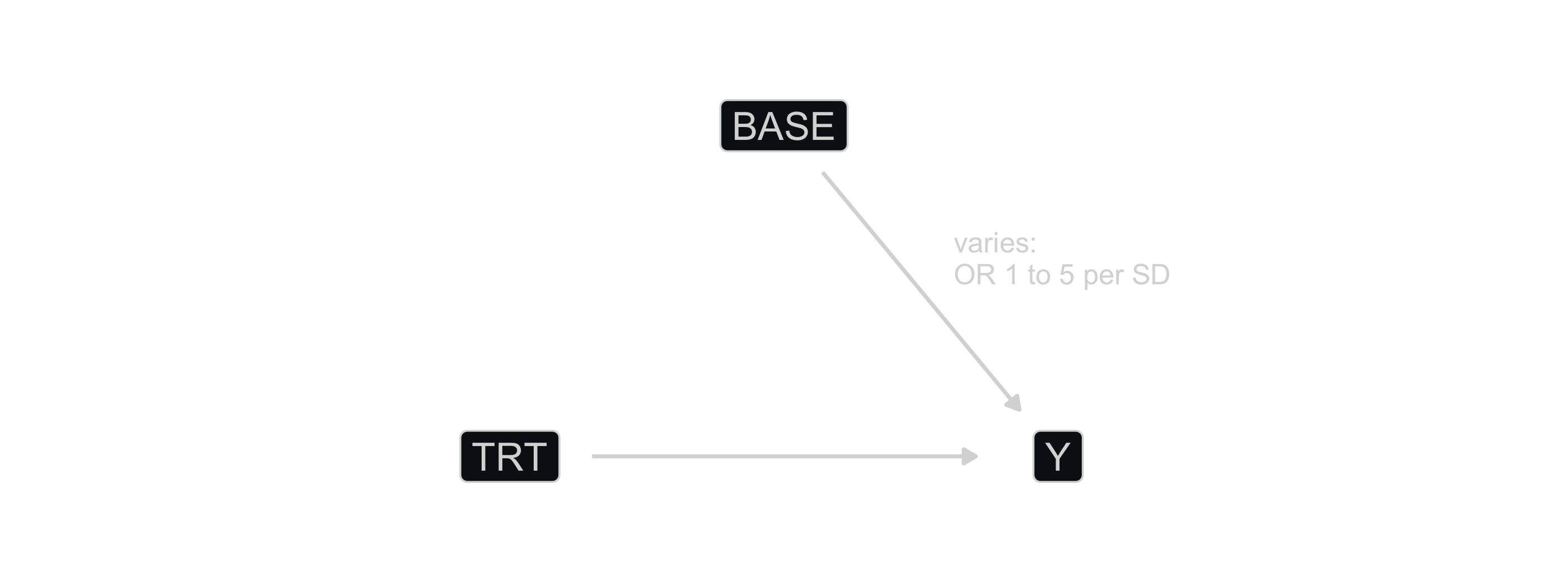
BASE affects the outcome but not the treatment received (no confounding).
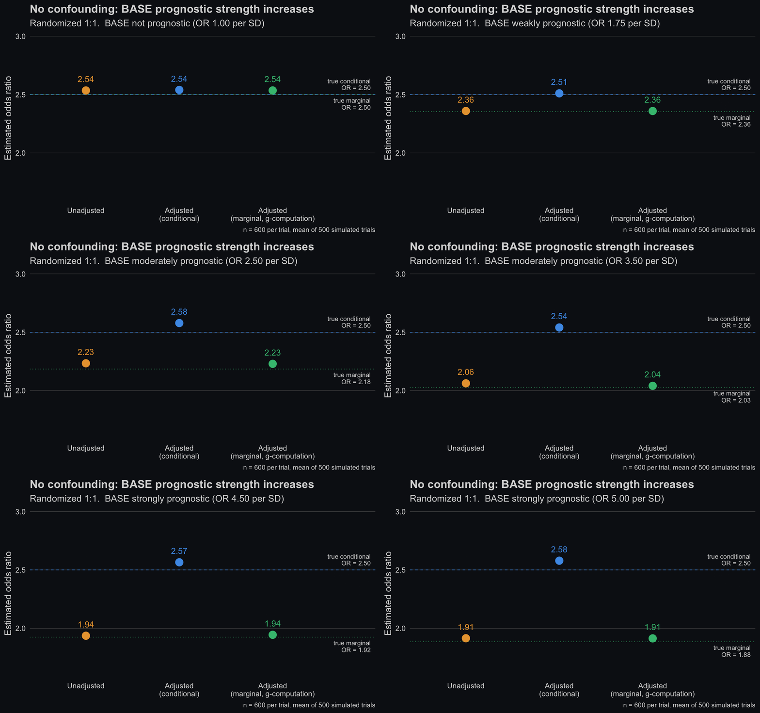
With no confounding, the unadjusted and the g-computation estimates stay together, and both move towards 1 as BASE becomes more prognostic. The adjusted coefficient stays at the conditional truth of 2.5.
Two of the three estimates move and one does not, and none of them is wrong! They are estimating different quantities. So the question is: what are you targeting?
Three estimates when assignment is confounded
BASE is now held at an odds ratio of 2.5 per standard deviation (it is prognostic), and what changes is how strongly BASE drives treatment assignment (confounding). At the first frame assignment is random. By the last frame patients with high BASE are much more likely to receive Active treatment.
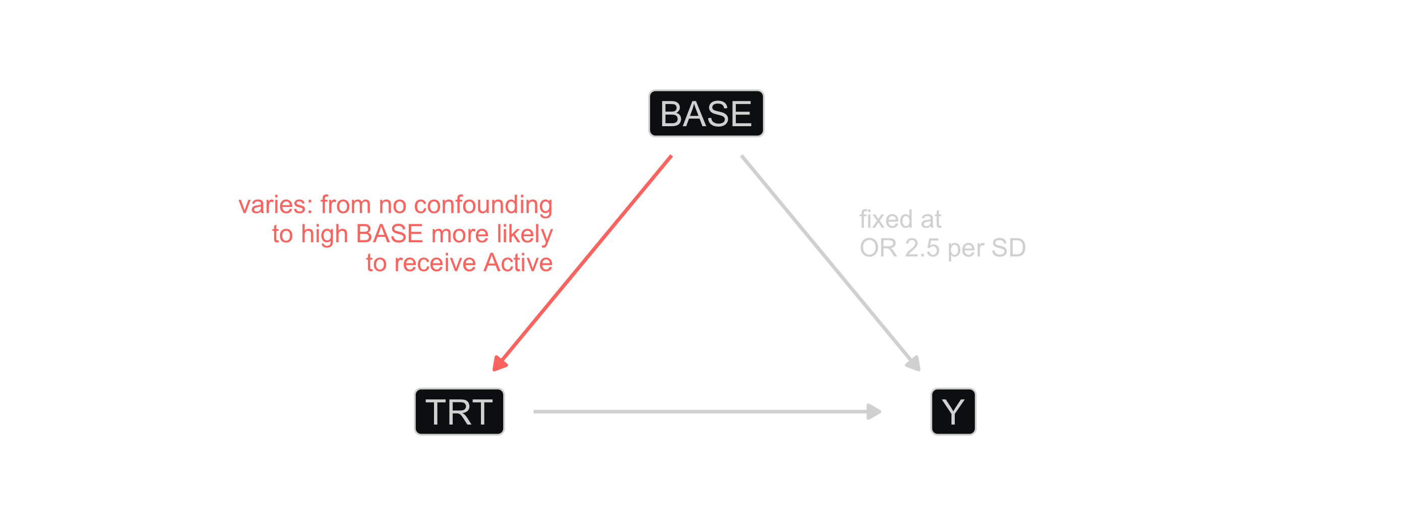
The only new arrow is BASE to TRT. BASE now points at both the treatment received and the outcome, which is what makes it a confounder.
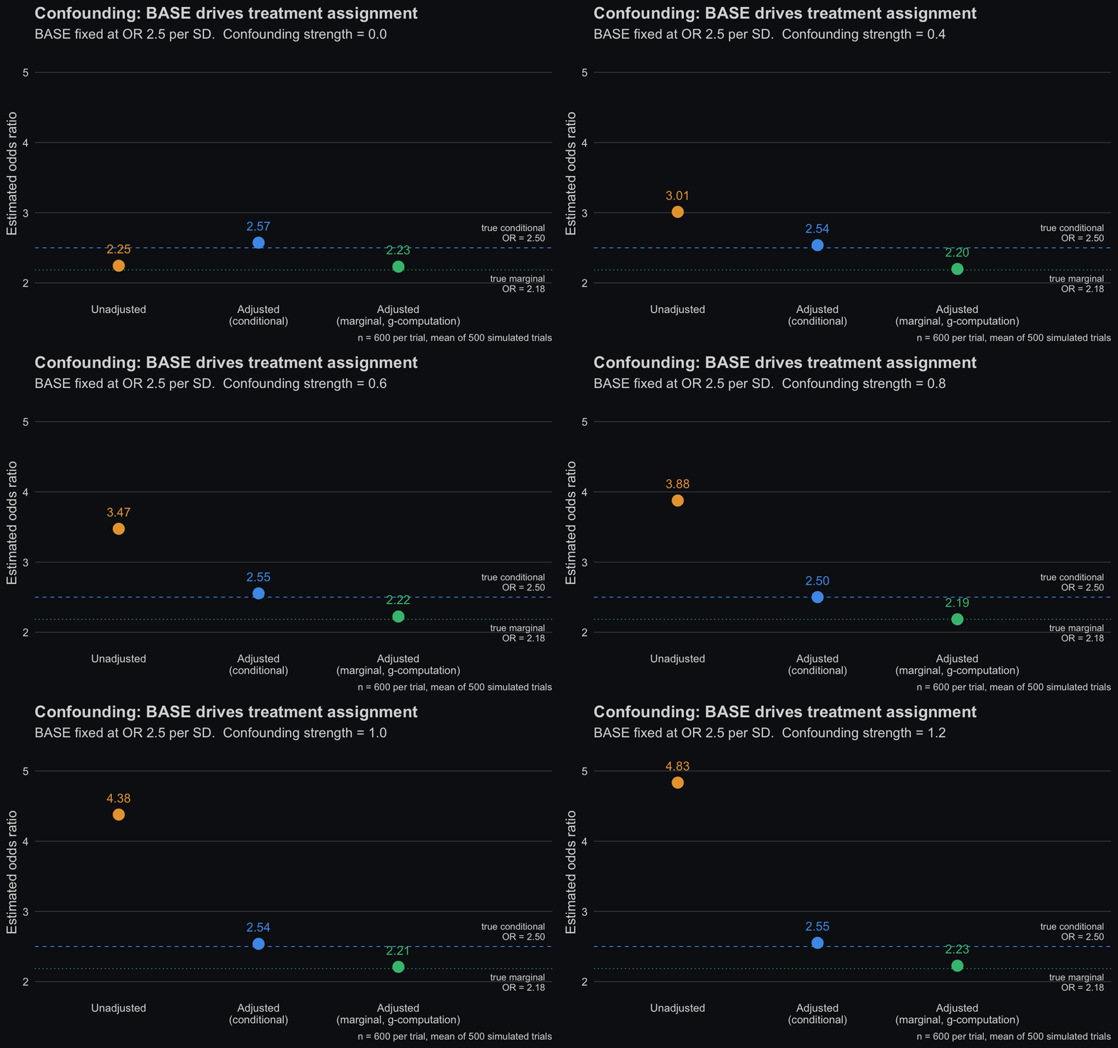
Now the unadjusted estimate is biased. It climbs away from both quantities taken from the adjusted model. Patients with high BASE are more likely to respond, and they are also more likely to receive Active. The Active arm fills up with patients who were going to do well anyway.
But be aware: G-computation is not magic either. It recovers the true marginal effect in our case only because the outcome model is correctly specified and BASE is the only confounder.😉
Conclusion
Adjusted or unadjusted is a choice about the model. Marginal or conditional is a choice about the estimand. One adjusted logistic model gives either one, depending on what is read out of it: the treatment coefficient is conditional, g-computation on the same fit is marginal.
When an unadjusted and an adjusted analysis disagree, there are two possible reasons, and they are commonly confused.
- Confounding. Treatment and the covariates are associated, so the unadjusted estimate does not recover the causal effect. Randomization handles it.
- Non-collapsibility. The conditional and the marginal OR are different quantities when the covariates predict the outcome and it happens even with perfect randomization.
So the choice has to be made and stated in advance, which is what the guidance asks for. Wei et al. give a fuller treatment of the two estimands and how to estimate them (Statistics in Biopharmaceutical Research 2024;16:371-381). Morris et al. are very useful on the same question, from the perspective of writing the analysis plan.
Back to the FDA review we started with. That study had repeated visits, and the review also discusses missing data, noting for instance that the GEE primary analysis assumed the data were missing completely at random (MCAR). An earlier post covers MCAR, MAR and MNAR if you want to dig into those. Those are real issues and they belong in your analysis plan. We left them out here on purpose, so that nothing moves in this post except the conditional and marginal distinction. Hope it helps! 😃