| Active | Control | Risk ratio | Odds ratio | |
|---|---|---|---|---|
| Common outcome | 45 / 100 (45.0%) | 25 / 100 (25.0%) | 1.80 | 2.45 |
| Rare outcome | 9 / 200 (4.5%) | 5 / 200 (2.5%) | 1.80 | 1.84 |
Odds ratio vs risk ratio: when they agree and when they don’t
Biostats
Estimands
Introduction
Odds ratios (ORs) are widely used to summarize binary outcomes, such as response versus no response or event versus no event. Risk ratios (RRs), also called relative risks, are also commonly reported.
An RR of 1.5 means the event is 1.5 times as likely in one group as in the other. An OR does not have that meaning, because it compares odds and not risks. At first glance, RRs may seem easier to interpret because they directly compare risks, but their interpretation is not always as straightforward as it appears, and they have important limitations 😐.
ORs and RRs are similar when the event is rare. They can be quite different when the event is common. Therefore, reporting or interpreting an OR as an RR can be misleading.
In this post we introduce ORs and RRs, show how they are calculated and interpreted, and show when they are similar and when they are different. We then look at how each one is estimated with a model, why the OR is used more often in clinical trials, and why converting an OR into a single RR is not always a good idea.
Everything below is a generic two-arm trial with a binary endpoint. The arms are Active and Control.
The two measures
With \(p_1\) the Active-arm response rate and \(p_0\) the Control-arm rate:
\[ \text{RR} = \frac{p_1}{p_0}, \qquad \text{OR} = \frac{p_1/(1-p_1)}{p_0/(1-p_0)} = \frac{a\,d}{b\,c} \]
where \(a\) and \(b\) are the Active-arm responders and non-responders, and \(c\) and \(d\) are the same for Control.
The RR divides one risk by the other. The OR divides one odds by the other. An odds is the chance of responding divided by the chance of not responding.
The table below shows the same RR at two different response levels.
The RR is 1.80 in both rows. The OR is not. It is 2.45 when the outcome is common and 1.84 when it is rare.
The difference comes from a single factor:
\[ \text{OR} = \text{RR} \times \frac{1-p_0}{1-p_1} \]
That factor is close to 1 only when both response rates are small. When the outcome is common, the OR is further from 1 than the RR.
When the two measures agree
Figure 1 shows how the relationship between the risk ratio (RR) and the odds ratio (OR) depends on the event rate in the Control arm. Starting with a given RR, we calculate the corresponding OR under two different scenarios: a low Control-arm rate of 5% and a higher rate of label_percent(accuracy = 1)(P0_HIGH)`. This allows us to compare the ORs produced by the same RR when the baseline risk differs. The dashed diagonal represents perfect agreement between the two measures—that is, the points at which the OR and RR have the same numerical value.
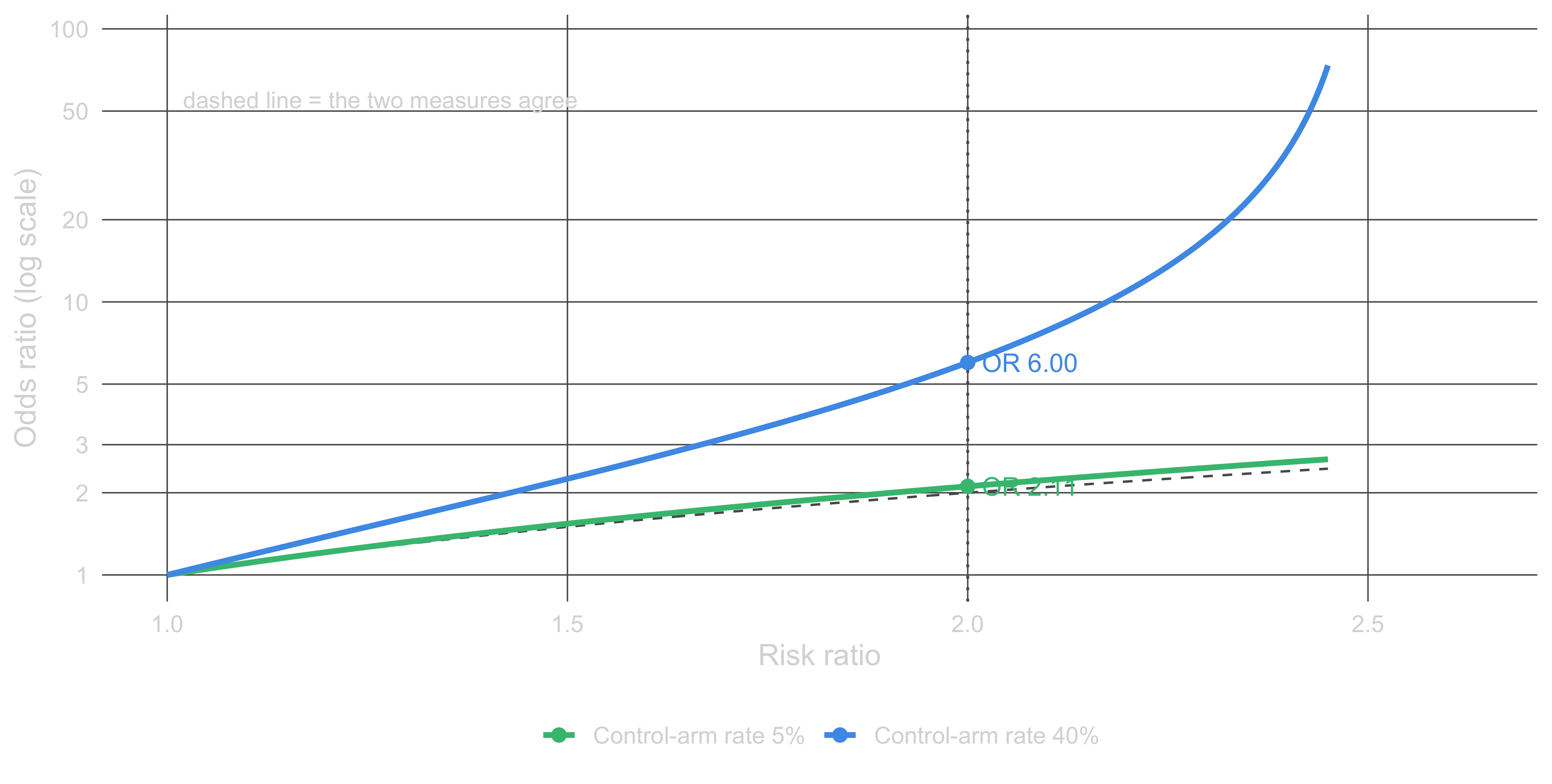
Take the dotted line at an RR of 2. With a 5% Control-arm rate, that benefit gives an OR of 2.11. The two numbers are close. With a 40% Control-arm rate, it gives an OR of 6.00. The two measures have different limits. The RR cannot go above \(1/p_0\), which is 20 and 2.5 for these two rates, because a response rate cannot go above 100%. The OR has no upper limit.
ORs and RRs agree only when the outcome is rare. McKenzie and Thomas suggest an incidence below about 10% as a working definition of rare (Eur J Clin Invest 2020;e13249). Cook argues that this is not a reason to avoid ORs when outcomes are common, but a reason to stop reading them as RRs (Acad Emerg Med 2002;9:1430-1434). Cook also says that the assumption of homogeneity of odds ratios is far more tenable in most situations than the implicit assumption of homogeneity of risk ratios. The apparent ease of application of risk ratios is negated by the fact that they are not as well understood as many believe, and naive applications may be incorrect.
Which measure is the bigger number
It is often said that the OR exaggerates the effect, meaning that it is the larger number. That is only half of the rule. Grant states that the OR is always further away from 1 than the RR (BMJ 2014;348:f7450). So the OR is the larger number when the treatment helps (assumming a response is defined as a favorable outcome), and the smaller number when it harms.
Figure 2 holds the Control-arm rate at 30% and moves the Active-arm rate across it, so all three cases appear in one panel.
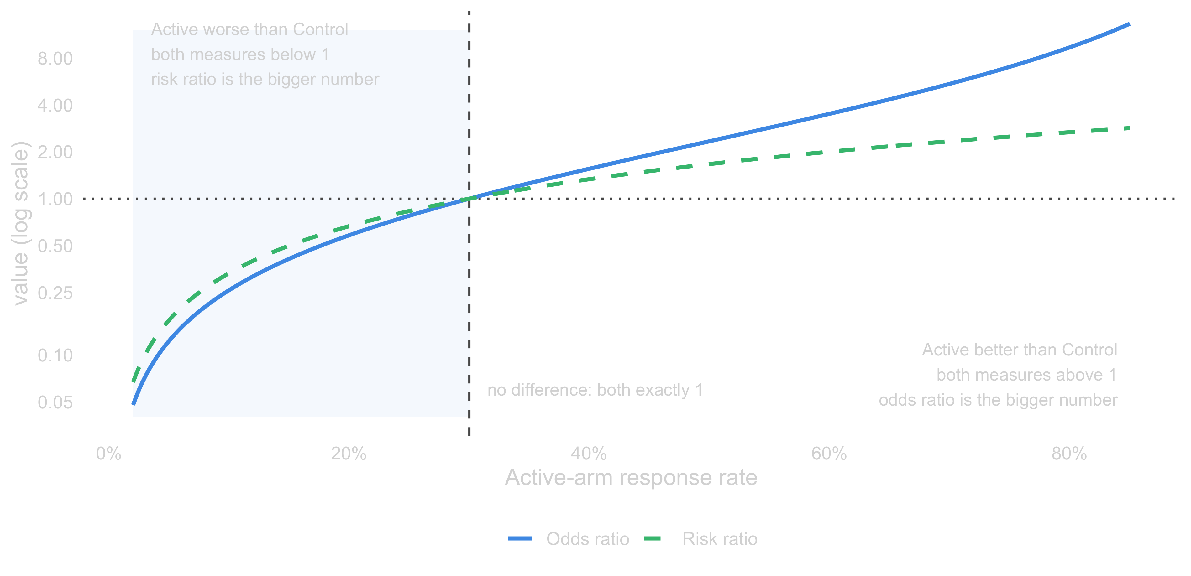
To the right of the dashed line more patients respond on Active. Both measures are above 1 and the OR is above the RR. To the left fewer patients respond on Active. Both measures are below 1 and the RR is now the larger number. On the line the two arms are identical and both measures equal 1.
So the RR can be larger than the OR, and this happens only when the OR is below 1.
Which measure does not change with baseline risk
The two sections above fixed the response rates. Figure 3 does the opposite. We fix the OR and ask what the RR would be in populations with a different baseline risk. The treatment effect stays the same, only the patients are sicker or healthier. The curve follows the standard conversion formula, \(\text{RR} = \text{OR}/(1-p_0+p_0\!\times\!\text{OR})\), read as a function of \(p_0\).
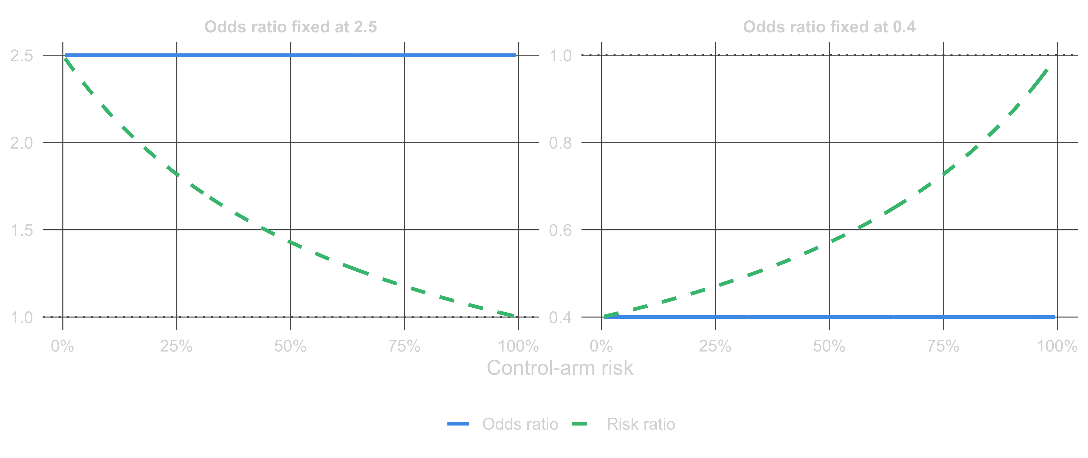
With the OR fixed at 2.5, the RR falls from 2.46 where 1% of controls respond, to 1.43 at 50%, and to 1.06 at 90%. Nothing about the treatment changed. The right panel shows the same drift for an OR < 1.
The reason is a limit on what a risk can be. A risk cannot go above 100%, and that puts a ceiling on the RR. If a treatment doubles the risk of an event, that cannot apply to a patient whose baseline risk is 60%, because it would imply a risk of 120%. The highest RR available at a baseline risk of \(p_0\) is \(1/p_0\), so the ceiling comes down as the baseline risk goes up.
This does not mean the OR is automatically constant across populations. It means a constant OR is possible, while a constant RR stops being possible once baseline risks vary widely. Doi and colleagues put the conclusion in their title: the OR is portable across baseline risk and the RR is not. They mention that “the OR should replace the RR in clinical research and meta-analyses though there should be conversion of the end product into ratios or differences of risk, solely, for interpretation”, “that RR depends on prevalence more so than on the strength of the exposure-outcome association that it is supposed to reflect” (J Clin Epidemiol 2022;142:288-293). Their view of the OR follows from that: it “measures solely the effect magnitude and has no relationship to the prevalence of an outcome in a study nor does it overestimate the RR as is commonly thought” (J Clin Epidemiol 2022;142:271-279).
Cook also writes that “the assumption of homogeneity of ORs is a more tenable assumption than the assumption of homogeneity of RRs and thus it is more likely that an estimate of the OR can be reliably applied to all individuals within a population”.
Estimating each measure with a model
So far we have only used 2x2 tables. In a real trial we fit a model, usually to adjust for baseline covariates.
Both options are generalized linear models (GLMs). A GLM connects the expected outcome to a linear predictor through a link function \(g\):
\[ g\!\left(E[Y]\right) = \beta_0 + \beta_1 x_1 + \dots + \beta_k x_k \]
The link function is what differs between the two models, and it is what decides which measure comes out. GLMs are covered in more detail in an earlier post.
- Logistic regression uses the logit link, \(g(p) = \log\!\left(p/(1-p)\right)\), and gives an OR.
- Log-binomial regression uses the log link, \(g(p) = \log(p)\), and gives an RR.
The two links are not equally easy to fit. A logistic model returns a probability between 0 and 1 for any value of its coefficients, so it converges almost always. A log link does not have that property. The fitted risk is the exponential of the linear predictor, and it must stay below 1, so the linear predictor must stay below 0. That constraint puts the best fit on or near the boundary of the parameter space, and standard software then reports failed convergence.
For this reason RRs are often estimated with modified Poisson regression with robust variance instead. Chen and colleagues compared the two approaches under model misspecification and found log-binomial point estimates to be biased where robust Poisson estimates were not (BMC Med Res Methodol 2018;18:63).
There is one more point worth making here. A logistic model gives fitted probabilities through the inverse link, so it is tempting to recover \(p_1\) and \(p_0\) and compute an RR from them. That can be done, but the RR you get depends on the baseline risk you use. Grant puts it directly: “any statistical model which contains a single odds ratio that is constant for all covariate values does not imply a constant relative risk, so to communicate relative risks effectively it is essential to provide a range of relative risks for different covariate values”.
Non-collapsibility, in two sentences
A measure is collapsible if its value in the whole population is a weighted average of its values in the subgroups. The RR is collapsible and the OR is not, which means the OR for the whole population differs from the OR within covariate subgroups, even in a randomized trial with no confounding. Neither number is wrong. That is the subject of the next post 😬.
FDA’s guidance on covariate adjustment makes the same distinction. It notes that “unlike the odds ratio or hazard ratio, the risk difference and relative risk are collapsible”, and asks sponsors to “specify whether the treatment effect of interest in an analysis is a conditional or unconditional treatment effect” (FDA, May 2023).
Conclusion
At first glance the RR is the more interpretable measure, and that is a fair point. “1.5 times as likely” is understood by everyone. But the OR has real advantages, and they explain why it is used more often:
- It keeps the same value across patients with different baseline risk, so one estimate applies at any level of risk.
- Its model fits reliably, including with covariate adjustment.
- It is available in case-control designs, where risks cannot be estimated at all.
The costs are real too. The OR is harder to explain, it is not collapsible, and it is easy to misread as an RR.
Our focus here has been randomized clinical trials. The argument for the OR is stronger still in meta-analysis. Trials enrol populations with different baseline risks, so pooling RRs combines numbers that are not directly comparable, while pooling ORs does not have that problem.
Neither measure is better in general. What matters is stating which one was used and interpreting it as what it is.